Learn how to use SQL to query TileDB-SOMA experiments.
Note
TileDB’s SQL query support is now provided by TileDB Tables. The TileDB storage engine for MariaDB, imported as tiledb.sql, and also known as MyTile or TileDB-MariaDB, is now deprecated.
How to run this tutorial
You can run this tutorial only on TileDB Cloud. However, TileDB Cloud has a free tier. We strongly recommend that you sign up and run everything there, as that requires no installations or deployment.
TileDB Cloud’s serverless SQL capability supports running SQL queries directly on TileDB arrays. This tutorial shows how to leverage this feature to interact with SOMA experiments. You will learn how to perform queries that filter, aggregate, and transform the data in a way that should be familiar to any SQL afficionados.
import osimport matplotlib.pyplot as pltimport pandas as pdimport seaborn as snsimport tiledbimport tiledb.cloudimport tiledbsomaimport tiledbsoma.iotiledbsoma.show_package_versions()
tiledbsoma.__version__              1.11.4
TileDB-Py version                   0.29.0
TileDB core version (tiledb)        2.23.1
TileDB core version (libtiledbsoma) 2.23.1
python version                      3.9.19.final.0
OS version                          Linux 6.8.0-1013-aws
Dataset
This tutorial uses a dataset from the Tabula Sapiens consortium, which includes nearly 265,000 immune cells across various tissue types. The original H5AD file was downloaded from Figshare and converted into a SOMA experiment using the TileDB-SOMA API. The resulting SOMA experiment is hosted on TileDB Cloud (tabula-sapiens-immune).
This SOMA experiment is accessible programmatically using the following URI:
Querying any of the underlying arrays within a SOMA experiment requires providing a URI, which you can retrieve with the tiledbsoma package. Start by opening the SOMA experiment:
The tiledb.sql.execute() function enables executing SQL queries on the array without managing any underlying infrastructure. The function always returns a pandas DataFrame containing the query results.
query =f"SELECT * FROM `{var_uri}`"df_var = tiledb.cloud.sql.exec(query)df_var
soma_joinid
feature_name
std
mean
feature_reference
feature_biotype
highly_variable
dispersions_norm
ensemblid
dispersions
feature_type
feature_is_filtered
means
gene_id
0
0
DDX11L1
0.005574
0.000039
NCBITaxon:9606
gene
0
-0.573947
ENSG00000223972.5
0.835044
Gene Expression
0
6.398244e-05
ENSG00000223972
1
1
WASH7P
0.031731
0.001080
NCBITaxon:9606
gene
0
0.533203
ENSG00000227232.5
2.442280
Gene Expression
0
2.274395e-03
ENSG00000227232
2
2
MIR6859-1
0.005634
0.000033
NCBITaxon:9606
gene
0
-0.256874
ENSG00000278267.1
1.295335
Gene Expression
0
6.175251e-05
ENSG00000278267
3
3
MIR1302-2HG
0.008041
0.000048
NCBITaxon:9606
gene
0
0.680668
ENSG00000243485.5
2.656352
Gene Expression
0
1.372886e-04
ENSG00000243485
4
4
MIR1302-2
1.000000
0.000000
NCBITaxon:9606
gene
0
0.000000
ENSG00000284332.1
0.000000
Gene Expression
0
1.000000e-12
ENSG00000284332
...
...
...
...
...
...
...
...
...
...
...
...
...
...
...
58554
58554
MT-ND6
0.741395
0.590065
NCBITaxon:9606
gene
0
0.154140
ENSG00000198695.2
2.466404
Gene Expression
0
9.634841e-01
ENSG00000198695
58555
58555
MT-TE
0.301820
0.083929
NCBITaxon:9606
gene
0
-0.044396
ENSG00000210194.1
1.603787
Gene Expression
0
1.600667e-01
ENSG00000210194
58556
58556
MT-CYB
1.104192
3.874830
NCBITaxon:9606
gene
0
-0.499747
ENSG00000198727.2
4.765751
Gene Expression
0
4.367693e+00
ENSG00000198727
58557
58557
MT-TT
0.186848
0.040580
NCBITaxon:9606
gene
0
-0.719108
ENSG00000210195.2
0.624316
Gene Expression
0
6.573967e-02
ENSG00000210195
58558
58558
MT-TP
0.501265
0.204806
NCBITaxon:9606
gene
1
1.115482
ENSG00000210196.2
2.705558
Gene Expression
0
4.385102e-01
ENSG00000210196
58559 rows × 14 columns
Filter
Filter the data using the WHERE clause in the SQL query. For instance, the following snippet filters the obs array to retrieve cell type annotations for all cells collected from Asian males.
query =f"""SELECT soma_joinid, cell_typeFROM `{experiment.obs.uri}`WHERE sex = 'male' AND ethnicity = 'Asian'"""df_obs = tiledb.cloud.sql.exec(query)df_obs
soma_joinid
cell_type
0
63240
monocyte
1
63241
monocyte
2
63242
plasma cell
3
63243
monocyte
4
63244
hematopoietic stem cell
...
...
...
2483
70996
hematopoietic stem cell
2484
70997
hematopoietic stem cell
2485
70998
plasma cell
2486
70999
hematopoietic stem cell
2487
71000
plasma cell
2488 rows × 2 columns
Full ANSI SQL is supported, so you can use complex queries to filter the data as needed.
Aggregate
Perform data aggregations using the GROUP BY clause in the SQL query.
This example calculates the mean and standard deviation of gene expression values across the subset of cells defined by the previous obs query. A HAVING clause filters out genes with fewer than 10 contributing cells to improve the robustness of the summaries.
query =f"""SELECT soma_dim_1, AVG(`soma_data`) AS avg, STD(`soma_data`) AS sd, COUNT(`soma_data`) AS n_cellsFROM `{experiment.ms["RNA"].X["data"].uri}`WHERE soma_dim_0 IN ({",".join(["?"] *len(df_obs))})GROUP BY soma_dim_1HAVING COUNT(`soma_dim_1`) >= 100"""result = tiledb.cloud.sql.exec(query, parameters=df_obs.soma_joinid.to_list())# Join with var to get feature namesresult.set_index("soma_dim_1").join(df_var.set_index("soma_joinid")[["feature_name"]])
avg
sd
n_cells
feature_name
soma_dim_1
1
2.961967
3.619777
130
WASH7P
19
4.578913
4.211768
155
WASH9P
32
0.144629
0.282825
391
MTND1P23
33
1.099287
1.039835
704
MTND2P28
34
0.558262
0.631345
725
MTCO1P12
...
...
...
...
...
58553
2.525545
0.886761
2274
MT-ND5
58554
2.138958
0.944408
1960
MT-ND6
58555
1.095660
1.450418
403
MT-TE
58556
3.147116
0.919982
2261
MT-CYB
58558
1.076467
1.181263
446
MT-TP
11448 rows × 4 columns
Distributed SQL queries
So far, the serverless SQL examples have all been executed on a single node. However, TileDB Cloud also supports distributed SQL queries, which scale operations by executing them across multiple nodes in parallel, speeding up processing for large datasets.
Construct a task graph composed of multiple nodes (i.e., SQL queries) that can be executed in parallel.
Tip
For more information on constructing and executing serverless pipelines, visit the Task Graphs section.
To see how this works, extend the previous aggregation example to calculate the gene-wise summary statistics within each cell type. Use a task graph to distribute the computations across each of the n cell types. Start by splitting the cell soma_joinid values into groups based on the cell_type column.
for cell_type, obs_ids in obs_ids_by_cell_type.items(): query =f""" SELECT soma_dim_1, AVG(`soma_data`) AS avg, STD(`soma_data`) AS sd, COUNT(`soma_data`) AS n_cells FROM `{experiment.ms["RNA"].X["data"].uri}` WHERE soma_dim_0 IN ({",".join(["?"] *len(obs_ids))}) GROUP BY soma_dim_1 HAVING COUNT(`soma_dim_1`) >= 20 """ graph.submit_sql(query, name=cell_type, parameters=obs_ids)# Visualize the task graphgraph.visualize()
Execute the SQL queries across all nodes by calling the task graph’s compute() method.
Once all nodes complete, retrieve the results. The output of the task graph is a Python dictionary where the keys are the cell type names and the values are the corresponding DataFrame objects.
result = ( pd.concat([df.assign(cell_type=name) for name, df in results.items()]) .set_index("soma_dim_1") .join(df_var.set_index("soma_joinid")[["feature_name"]]))result
avg
sd
n_cells
cell_type
feature_name
soma_dim_1
32
0.133643
0.284189
26
CD4-positive, alpha-beta T cell
MTND1P23
33
1.382537
1.058097
100
CD4-positive, alpha-beta T cell
MTND2P28
34
0.528415
0.707839
106
CD4-positive, alpha-beta T cell
MTCO1P12
36
1.687168
2.084468
86
CD4-positive, alpha-beta T cell
MTCO2P12
38
1.136198
0.426818
400
CD4-positive, alpha-beta T cell
MTATP6P1
...
...
...
...
...
...
58553
2.731793
0.848978
371
plasma cell
MT-ND5
58554
2.055919
0.980311
368
plasma cell
MT-ND6
58555
0.293131
0.305294
136
plasma cell
MT-TE
58556
3.074683
0.838316
372
plasma cell
MT-CYB
58558
0.503710
0.460197
153
plasma cell
MT-TP
66467 rows × 5 columns
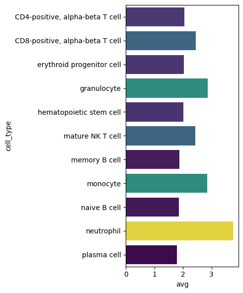
Visualize the expression profile for any given gene across different cell types to compare how the gene behaves in various cellular contexts.
GENE_SYMBOL ="MYL6"plt.figure(figsize=(5, 6))# Create the bar plotsns.barplot( data=result.query(f"feature_name == '{GENE_SYMBOL}'"), x="avg", y="cell_type", hue="avg", palette="viridis", legend=False,)plt.tight_layout()# Show the plotplt.show()
Summary
This tutorial covered how to run SQL queries on TileDB-SOMA experiments using TileDB Cloud and how to scale these operations efficiently with Task Graphs. For additional examples and information on Task Graphs, explore the SOMA Distributed Compute tutorial.