Learn how to access TileDB-SOMA data in a variety of ways.
This tutorial outlines how to access single-cell data stored in a SOMA experiment. See the Data Ingestion tutorial for information on how to create a SOMA experiment from a single-cell dataset.
Prerequisites
While you can run this tutorial locally, note that this tutorial relies on remote resources to run correctly.
You must create a REST API token and create an environment variable named $TILEDB_REST_TOKEN set to the value of your generated token.
Setup
First, load tiledbsoma as well as a few other packages used in this tutorial:
import scanpy as scimport tiledbsomaimport tiledbsoma.iotiledbsoma.show_package_versions()
tiledbsoma.__version__              1.11.4
TileDB-Py version                   0.29.0
TileDB core version (tiledb)        2.23.1
TileDB core version (libtiledbsoma) 2.23.1
python version                      3.9.19.final.0
OS version                          Linux 6.8.0-1013-aws
tiledbsoma:    1.11.4
tiledb-r:      0.27.0
tiledb core:   2.23.1
libtiledbsoma: 2.23.1
R:             R version 4.3.3 (2024-02-29)
OS:            Debian GNU/Linux 11 (bullseye)
Dataset
This tutorial uses a dataset from the Tabula Sapiens consortium, which includes nearly 265,000 immune cells across various tissue types. The original H5AD file was downloaded from Figshare and converted into a SOMA experiment using the TileDB-SOMA API. The resulting SOMA experiment is hosted on TileDB Cloud (tabula-sapiens-immune).
This SOMA experiment is accessible programmatically with the following URI:
Note that opening a SOMA experiment (or any SOMA object) only returns a pointer to the object on disk. No data is actually loaded into memory until it’s requested.
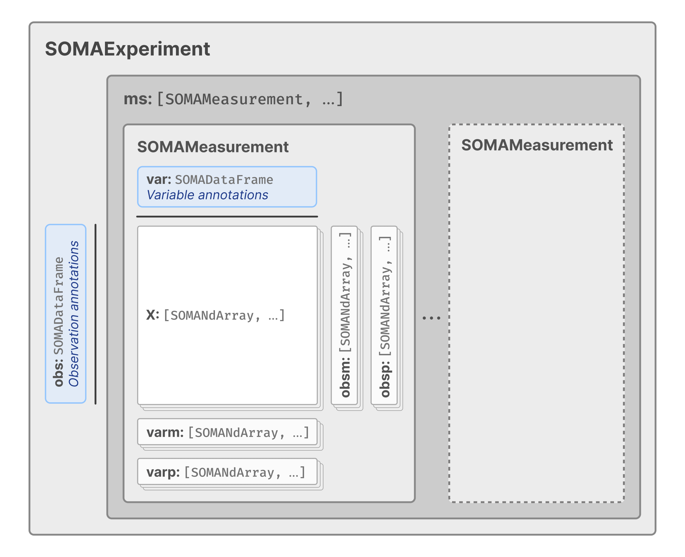
The top level of the experiment contains two elements: obs, a SOMA DataFrame containing the cell annotations; and ms, a SOMA Collection of the measurements (e.g., RNA) in the experiment.
Other elements are nested within the experiment according to the SOMA data model (see the following diagram) but are accessible using a similar syntax.
For example, feature-level annotations are stored in the var array, which is always located at the top-level of each SOMA Measurement. This dataset contains only a single measurement, RNA but more complex datasets may contain multiple measurements. Access the RNA measurement’s var array.
Similarly, assay data (e.g., RNA expression levels) is stored in SOMASparseNDArrays within the X collection. Each array within X is referred to as a layer. Access the X collection to see what layers are available.
The next section covers reading data from these components.
Read into memory
All array-based SOMA objects provide a read method for loading data into memory. Designed with large datasets in mind, these methods always return an iterator, allowing data to be loaded in chunks intelligently sized by TileDB to accommodate the allocated memory, and efficiently materialize the results in Apache Arrow format, leveraging zero-copy memory sharing where possible.
In following example, expression values from the Xdata layer are loaded into memory one chunk at a time.
The .tables() method is used to materialize each chunk as an Arrow Table. For the sake of this tutorial, the operation is limited to the first 3 chunks.
chunks = []for chunk in experiment.ms["RNA"].X["data"].read().tables():iflen(chunks) ==3:break chunks.append(chunk)chunks
[[1]]
Table
2097152 rows x 3 columns
$soma_dim_0 <int64 not null>
$soma_dim_1 <int64 not null>
$soma_data <float not null>

[[2]]
Table
2097152 rows x 3 columns
$soma_dim_0 <int64 not null>
$soma_dim_1 <int64 not null>
$soma_data <float not null>

[[3]]
Table
2097152 rows x 3 columns
$soma_dim_0 <int64 not null>
$soma_dim_1 <int64 not null>
$soma_data <float not null>
This approach is particularly useful when working with large arrays that may not fit into memory all at once. However, for smaller arrays that comfortably fit into memory, the concat method is used to automatically load all chunks and concatenate them into a single Arrow Table.
One of the most useful features of SOMA is the ability to efficiently select and filter only the data necessary for your analysis without loading the entire dataset into memory first. The read methods offer several arguments to access a specific subset of data, depending on the type of object being read.
The most basic type of filtering is selecting a subset of records based on their coordinates using the coords argument, which is available on all array-based SOMA objects.
This example loads the expression data for the first 100 cells and 50 genes. Because the requested slice is realtively small the .concat() method is added to return a single Arrow Table before converting the output to a pandas DataFrame.
This example loads the expression data for the first 100 cells and 50 genes. Because the requested slice is realtively small the $concat() method is added to return a single Arrow Table before converting the output to a data.frame.
For SOMADataFrame objects like obs and var, the read method provides additional arguments to filter by values on query conditions and select a subset of columns to return.
Load the first 100 records from obs with at least 2,000 detected reads and retrieve only two columns of interest from the array.
Leverage the same filtering options on the var array to retrieve pre-calculated gene expression means and standard deviations for a set of relevant genes.
For SOMASparseNDArrays such as X layers containing expression data (for this dataset) or obsm layers containing dimensionality reduction results, the read method’s filtering capabilities are limited to the coords argument.
This example loads expression data for the first 100 cells and 50 genes as a table.
The real power of the SOMA API comes from the ability to slice and filter measurement data based on the cell- and feature-level annotations stored in the experiment. For datasets containing millions of cells, this means you can easily access expression values for cells within a specific cluster, or that meet a certain quality threshold, etc.
The example below shows how to filter for highly variable genes within dendritic cells.
The returned query object allows you to inspect the query results and selectively access data. For example, you can see how many cells and genes were returned by the query:
Data loaded into memory from a SOMA experiment via the query object only includes records that matches the specified query criteria. The following example demonstrates how to load expression values for matching cells and genes from an X layer.
Note the shape of the returned tensor corresponds to the capacity of the underlying TileDB array. By default, SOMA creates arrays with extra room for adding new data in the future.
From here, you could use the to_sparse_matrix() method to easily load query results for any matrix-like data as a sparse dgTMatrix (from the Matrix package). At a minimum, you need to pass a collection (e.g., X, or obsm) and layer (e.g., data). You can also populate the matrix dimension names by specifying which obs column contains the values to use for row names and which var column contains the values to use for column names.
mat <- query$to_sparse_matrix(collection ="X",layer_name ="data",obs_index ="cell_id",var_index ="var_id")mat[1:10, 1:5]
SOMA also provides support for exporting query results to various in-memory data structures used by popular single-cell analysis toolkits. As before, the results only include data that passed the specified query criteria. Unlike the query accessors shown previously, these methods must access and load multiple data elements to construct these complex objects but still offer flexibility to customize what is included in the resulting object.
This example shows how to materialize the query results as an Seurat object, populating the RNA Assay’s data slot with expression data from the data layer. The obs_index and var_index arguments are used to specify which columns in the obs and var arrays should be used as column and row names, respectively.
An object of class Seurat
2435 features across 533 samples within 1 assay
Active assay: RNA (2435 features, 0 variable features)
 1 layer present: data
Now that you have the data loaded in memory and in a toolkit-specific format, the full suite of analysis and visualization methods provided by that toolkit are available.
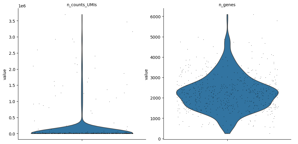
This example leverages scanpy’s plotting capabilities to visualize the distribution of the n_counts_UMIs and n_genes attributes across the cells in the query result.
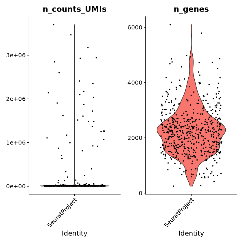
This example leverages Seurat’s plotting capabilities to visualize the distribution of the n_counts_UMIs and n_genes attributes across the cells in the query result.
Seurat::VlnPlot(sobj, features =c("n_counts_UMIs", "n_genes"))