API Usage

Learn about different examples of using the TileDB APIs with task graphs.

This document guides you through different examples of the TileDB task graph APIs. You can combine one or more Delayed objects into a task graph, which is typically a directed acyclic graph (DAG). You can pass the output from one function or query into another, and TileDB automatically calculates the dependencies for you.

Generic functions

The following code snippet shows a basic task graph that finds the median value of a list of numbers.

Python

import numpy
from tiledb.cloud.compute import Delayed

# Wrap numpy median in a delayed object
x = Delayed(numpy.median)

# It can be called like a normal function to set the parameters
# Note at this point the function does not get executed since it
# is of "delayed" type
x([1, 2, 3, 4, 5])

# To force execution and get the result call `compute()`
print(x.compute())

3.0

R

library(tiledbcloud)

# Wrap median in a delayed object
x <- delayed(median)

# You can set the parameters.  Note at this point the function does not
# get executed since it # is of "delayed" type.
delayed_args(x) <- list(c(1, 2, 3, 4, 5))

# To force execution and get the result call `compute()`
print(compute(x))

[1] 3

SQL and arrays

Besides arbitrary Python/R functions, you can also call serverless SQL queries and array UDFs with the delayed API.

Here’s an example of serverless SQL:

Python

from tiledb.cloud.compute import DelayedSQL

y = DelayedSQL("select AVG(`a`) FROM `tiledb://TileDB-Inc/quickstart_sparse`")

# Run query
print(y.compute())

   AVG(`a`)
0       2.0

R

library(tiledbcloud)

y <- delayed_sql("select AVG(`a`) FROM `tiledb://TileDB-Inc/quickstart_sparse`")

# Run query
print(compute(y))

  AVG(`a`)
1   2.0000

Here’s an example of array UDFs:

Python

import numpy
from tiledb.cloud.compute import DelayedArrayUDF

z = DelayedArrayUDF(
    "tiledb://TileDB-Inc/quickstart_sparse", lambda x: numpy.average(x["a"])
)([(1, 4), (1, 4)])

# Run the UDF on the array
print(z.compute())

2.0

R

library(tiledbcloud)

z <- delayed_array_udf(
  "tiledb://TileDB-Inc/quickstart_sparse",
  function(x) mean(x[["a"]]),
  selectedRanges = list(cbind(1, 4), cbind(1, 4)),
  attrs = c("a")
)

# Run the UDF on the array
print(compute(z))

[1] 2

Local functions

You can also specify a generic Python function as delayed, but have it run locally instead of serverless on TileDB Cloud. This is useful for testing or for saving final results to your local machine (for example, saving an image).

Python

import numpy
from tiledb.cloud.compute import Delayed

# Set the `local` argument to `True`
local = Delayed(numpy.median, local=True)([1, 2, 3])

# This will compute locally
local.compute()

2.0

R

library(tiledbcloud)

# Wrap median in a delayed object
x <- delayed(median)

# You can set the parameters.  Note at this point the function does not
# get executed since it # is of "delayed" type.
delayed_args(x) <- list(c(1, 2, 3))

# To force execution and get the result call `compute()`
print(compute(x, force_all_local = TRUE))

[1] 2

Heterogeneous task graphs

You can create task graphs by mixing different resource configurations and programming languages. The following example combines generic UDFs, array UDFs, and serverless SQL queries into a single task graph:

Python

import numpy as np
from tiledb.cloud.compute import Delayed, DelayedArrayUDF, DelayedSQL

# Build several delayed objects to define a graph
# Note that package numpy is aliased as np in the UDFs
local_fn = Delayed(lambda x: x * 2, local=True)(100)
array_apply = DelayedArrayUDF(
    "tiledb://TileDB-Inc/quickstart_sparse", lambda x: sum(x["a"].tolist())
)([(1, 4), (1, 4)])
sql = DelayedSQL(
    "select SUM(`a`) as a from `tiledb://TileDB-Inc/quickstart_dense`", name="sql"
)


# Custom function for averaging all the results we are passing in
def mean(local_fn, array_apply, sql):
    return np.mean([local_fn, array_apply, sql.iloc[0, 0]])


# This is essentially a task graph that looks like
#                 mean
#          /       |      \
#         /        |       \
#      local  array_apply  sql
#
# The `local`, `array_apply` and `sql` tasks will computed first,
# and once all three are finished, `mean` will computed on their results
res = Delayed(mean, local_fn, array_apply, sql)
print(res.compute())

114.0

R

library(tiledbcloud)

# Build several delayed objects to define a graph

# Locally executed; simple enough
local <- delayed(function(x) {
  x * 2
}, local = TRUE)
delayed_args(local) <- list(100)

# Array UDF -- we specify selected ranges and attributes, then do some R on the
# dataframe which the UDF receives
array_apply <- delayed_array_udf(
  array = "TileDB-Inc/quickstart_sparse",
  udf = function(df) {
    sum(as.vector(df[["a"]]))
  },
  selectedRanges = list(cbind(1, 4), cbind(1, 4)),
  attrs = c("a")
)

# SQL -- note the output is a dataframe, and values are all strings (MariaDB
# "decimal values") so we'll cast them to numeric later
sql <- delayed_sql(
  "select SUM(`a`) as a from `tiledb://TileDB-Inc/quickstart_dense`",
  name = "sql"
)

# Custom function for averaging all the results we are passing in
ourmean <- function(local, array_apply, sql) {
  mean(c(local, array_apply, as.numeric(sql[["a"]])))
}

# This is essentially a task graph that looks like
#               ourmean
#          /       |      \
#         /        |       \
#      local  array_apply  sql
#
# The `local`, `array_apply` and `sql` tasks will computed first,
# and once all three are finished, `ourmean` will computed on their results.
# Note here we slot out the answer from the SQL dataframe using `[[...]]`,
# and also cast to numeric.
res <- delayed(ourmean, args = list(local, array_apply, sql))
print(compute(res, verbose = FALSE))

[1] 114

Register task graph

You can register task graphs in the TileDB catalog, so that you can search, share, and execute them without needing to build and have the code for the entire task graph in a local environment. You can call a registered task graph directly while passing input parameters into the task graph.

Python

# This is the same implementation which backs `Delayed`, but this interface
# is better suited to more advanced use cases where full control is desired.
graph = builder.TaskGraphBuilder(name="Registration Example")

# Define a graph
# Note that package numpy is aliased as np in the UDFs
l_func = graph.submit(lambda x: x * 2, 100, name="l_func")
array_apply = graph.array_udf(
    "tiledb://TileDB-Inc/quickstart_sparse",
    lambda x: np.sum(x["a"]),
    name="array_apply",
    ranges=[(1, 4), (1, 4)],
)
sql = graph.sql(
    "select SUM(`a`) as a from `tiledb://TileDB-Inc/quickstart_dense`", name="sql"
)


# Custom function for averaging all the results we are passing in
def mean(l_func, array_apply, sql):
    return np.mean([l_func, array_apply, sql.iloc(0)[0]])


# This is essentially a task graph that looks like
#                mean
#          /      |    \
#         /       |     \
#   l_func  array_apply  sql
#
# The `l_func`, `array_apply` and `sql` tasks will computed first,
# and once all three are finished, `mean` will computed on their results
res = graph.udf(
    func=mean,
    name="node_exec",
    types.args(l_func=l_func, array_apply=array_apply, sql=sql),
)

# Now let's register the dag instead of running it
tiledb.cloud.taskgraphs.register(dag, name="registration-example")

# To call the dag we simply load it, then execute.
new_tgb = tiledb.cloud.taskgraphs.registration.load(
    "registration-example", namespace="TileDB-Inc"
)
results = tiledb.cloud.taskgraphs.execute(new_tgb)

Modes of Operation

REALTIME

The default mode of operation, REALTIME, is designed to return results directly to the client, with an emphasis on low latency. Real-time task graphs are scheduled and executed immediately and are well-suited for fast, distributed workloads.

BATCH

In contrast to real-time task graphs, BATCH task graphs are designed for large, resource intensive asynchronous workloads. Batch task graphs are defined, uploaded, and scheduled for execution and are well suited for ingestion-style workloads.

Set the task graph mode

The mode can be set for any of the APIs by passing in a mode parameter. Accepted values are BATCH or REALTIME.

Delayed API mode

Python

import tiledb.cloud

batch_function = Delayed(numpy.median, mode=tiledb.cloud.dag.Mode.BATCH)

realtime_function = Delayed(numpy.median, mode=tiledb.cloud.dag.Mode.REALTIME)

DAG API mode

Python

batch_dag = tiledb.cloud.dag.DAG(mode=tiledb.cloud.dag.Mode.BATCH)

realtime_dag = tiledb.cloud.dag.DAG(mode=tiledb.cloud.dag.Mode.REALTIME)

Visualization

Any task graph created using the delayed API can be visualized with visualize(). The graph will be auto-updated by default as the computation progresses. If you wish to disable auto-updating, then set auto_update=False as a parameter in visualize(). If you are inside a Jupyter notebook, the graph will render as a widget. If you are not on the notebook, you can set notebook=False as a parameter to render in a normal Python window.

Python

res.visualize()

Retry functions

If a function fails or you cancel it, you can manually retry the given node with the .retry method, or retry all failed nodes in a DAG with .retry_all(). Each retry call retries a node once.

Python

from tiledb.cloud.compute import Delayed

# Retry one node:

flaky_node = Delayed(flaky_func)(my_data)
final_output = Delayed(process_output)(flaky_node)

data = final_output.compute()
# -> Raises an exception since flaky_node failed.

flaky_node.retry()
data = final_output.result()

# Retry many nodes:

flaky_inputs = [Delayed(flaky_func)(shard) for shard in input_shards]
combined = Delayed(merge_outputs)(flaky_inputs)

combined.compute()
# -> Raises an exception since some of the flaky inputs failed.

combined.dag.retry_all()
combined.dag.wait()

data = combined.result()

Cancel a task graph

If you have a running task graph, you can cancel it with the .cancel() function on the DAG or Delayed object.

Python

import tiledb.cloud


def my_func():
    import time

    time.sleep(120)
    return


batch_dag = tiledb.cloud.dag.DAG(mode=tiledb.cloud.dag.Mode.BATCH)
result = batch_dag.submit(my_func)
# Start task graph
batch_dag.compute()


# Cancel Task Graph
batch_dag.cancel()

Advanced Usage

Manually set delayed task dependencies

Sometimes, one function depends on another without directly using its results. A common case is when one function manipulates data stored somewhere else (on S3 or a database). To support this, TileDB has the depends_on function.

Python

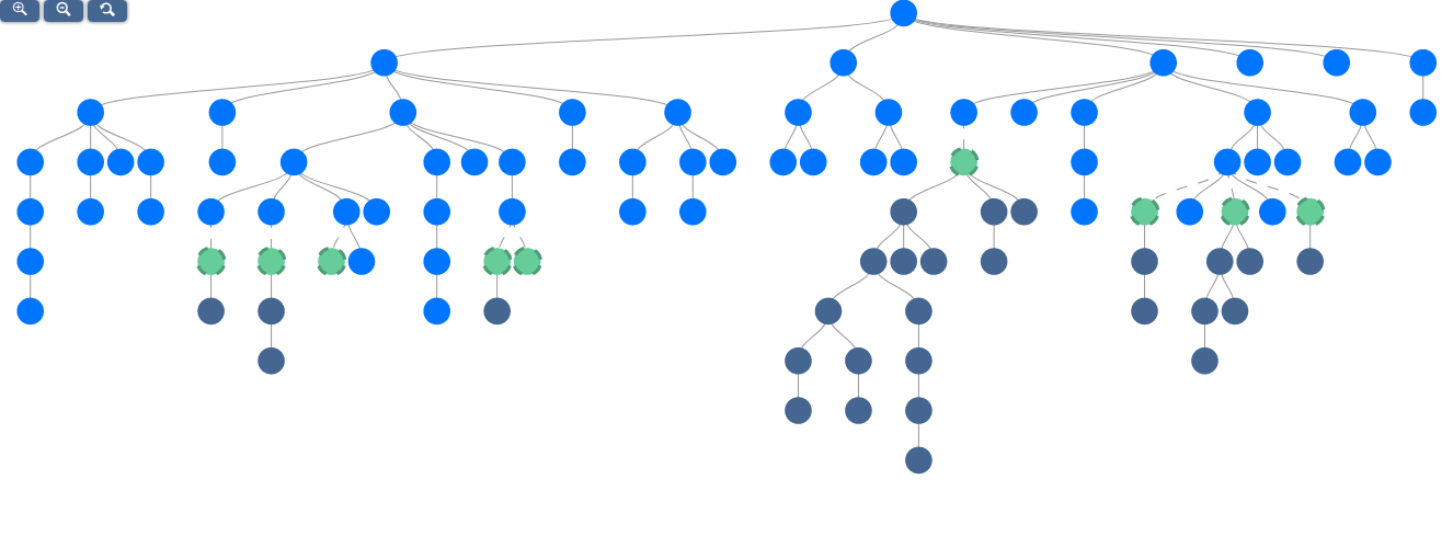
# A few base functions:
import random

from tiledb.cloud.compute import Delayed

# Set three initial nodes
node_1 = Delayed(numpy.median, local=True, name="node_1")([1, 2, 3])
node_2 = Delayed(lambda x: x * 2, local=True, name="node_2")(node_1)
node_3 = Delayed(lambda x: x * 2, local=True, name="node_3")(node_2)

# Create a dictionary to hold the nodes so we can randomly pick dependencies
nodes_by_name = {"node_1": node_1, "node_2": node_2, "node_3": node_3}


# Function which sleeps for some time so we can see the graph in different states
def f():
    import random
    import time

    time.sleep(random.randrange(0, 30))
    return x


# Randomly add 96 other nodes to the graph. All of these will use the sleep function
for i in range(4, 100):
    name = "node_{}".format(i)
    node = Delayed(f, local=True, name=name)()

    dep = random.randrange(1, i - 1)
    # Randomly set dependency on one other node
    node_dep = nodes_by_name["node_{}".format(dep)]
    # Force the dependency to be set
    node.depends_on(node_dep)

    nodes_by_name[name] = node

# Get the last function's results
node_99 = nodes_by_name["node_99"]
node_99.compute()

The above code, after the call to node_1.visualize(), produces a task graph similar to that shown below:

Low-level task graph API

TileDB provides a lower-level task graph API, which gives full control of building out arbitrary task graphs.

Python

import numpy as np
from tiledb.cloud.dag import dag

# This is the same implementation which backs `Delayed`, but this interface
# is better suited more advanced use cases where full control is desired.
graph = dag.DAG()

# Define a graph
# Note that package numpy is aliased as np in the UDFs
local_fn = graph.submit_local(lambda x: x * 2, 100)
array_apply = graph.submit_array_udf(
    "tiledb://TileDB-Inc/quickstart_sparse",
    lambda x: sum(x["a"].tolist()),
    name="array_apply",
    ranges=[(1, 4), (1, 4)],
)
sql = graph.submit_sql(
    "select SUM(`a`) as a from `tiledb://TileDB-Inc/quickstart_dense`"
)


# Custom function for averaging all the results we are passing in
def mean(local, array_apply, sql):
    return np.mean([local, array_apply, sql.iloc[0, 0]])


# This is essentially a task graph that looks like
#                 mean
#          /       |      \
#         /        |       \
#      local  array_apply  sql
#
# The `local`, `array_apply` and `sql` tasks will computed first,
# and once all three are finished, `mean` will computed on their results
res = graph.submit_udf(mean, local_fn, array_apply, sql)
graph.compute()
graph.wait()

print(res.result())

114.0

Select whom to charge

If you are a member of at least one organization, then by default, TileDB charges the first organization to which you belong your Delayed tasks. If you would like to charge the task to yourself, you just need to add one extra argument, namespace.

To set up your personal billing details, visit the Individual Billing section.

For details about TileDB’s charging policy for individuals who are members of multiple organizations, review the Charging Policy.

Python

import tiledb.cloud

res = DelayedSQL(
    "select `rows`, AVG(a) as avg_a from `tiledb://TileDB-Inc/quickstart_dense` GROUP BY `rows`",
    namespace=namespace_to_charge,  # who to charge the query to
)

# When using the Task Graph API set the namespace on the DAG object
dag = tiledb.cloud.dag.DAG(namespace=namespace_to_charge)
dag.submit_sql(
    "select `rows`, AVG(a) as avg_a from `tiledb://TileDB-Inc/quickstart_dense` GROUP BY `rows`"
)

R

library(tiledbcloud)

res <- delayed_sql(
  query = "select `rows`, AVG(a) as avg_a from `tiledb://TileDB-Inc/quickstart_dense` GROUP BY `rows`",
  namespace = namespace_to_charge
)
out <- compute(res)
str(out)

You can also set whom to charge for the entire task graph instead of individual Delayed objects. This is often useful when building a large task graph, to avoid having to set the extra parameter on every object. Taking the example above, you just pass namespace="my_username" to the compute call.

Python

import numpy as np
from tiledb.cloud.compute import Delayed, DelayedArrayUDF, DelayedSQL

# Build several delayed objects to define a graph
local_fn = Delayed(lambda x: x * 2, local=True)(100)
array_apply = DelayedArrayUDF(
    "tiledb://TileDB-Inc/quickstart_sparse",
    lambda x: sum(x["a"].tolist()),
    name="array_apply",
)([(1, 4), (1, 4)])
sql = DelayedSQL("select SUM(`a`) as a from `tiledb://TileDB-Inc/quickstart_dense`")


# Custom function to use to average all the results we are passing in
def mean(local, array_apply, sql):
    return np.mean([local, array_apply, sql.iloc[0, 0]])


res = Delayed(func_exec=mean, name="node_exec")(local_fn, array_apply, sql)

# Set all tasks to run under your username
print(res.compute(namespace=namespace_to_charge))

114.0

R

library(tiledbcloud)

# Build several delayed objects to define a graph

# Locally executed; simple enough
local <- delayed(function(x) {
  x * 2
}, local = TRUE)
delayed_args(local) <- list(100)

# Array UDF -- we specify selected ranges and attributes, then do some R on the
# dataframe which the UDF receives
array_apply <- delayed_array_udf(
  array = "TileDB-Inc/quickstart_dense",
  udf = function(df) {
    sum(as.vector(df[["a"]]))
  },
  selectedRanges = list(cbind(1, 4), cbind(1, 4)),
  attrs = c("a")
)

# SQL -- note the output is a dataframe, and values are all strings (MariaDB
# "decimal values") so we'll cast them to numeric later
sql <- delayed_sql(
  "select SUM(`a`) as a from `tiledb://TileDB-Inc/quickstart_dense`",
  name = "sql"
)

# Custom function for averaging all the results we are passing in
ourmean <- function(local, array_apply, sql) {
  mean(c(local, array_apply, sql))
}

# This is essentially a task graph that looks like
#               ourmean
#          /       |      \
#         /        |       \
#      local  array_apply  sql
#
# The `local`, `array_apply` and `sql` tasks will computed first,
# and once all three are finished, `ourmean` will computed on their results.
# Note here we slot out the answer from the SQL dataframe using `[[...]]`,
# and also cast to numeric.
res <- delayed(ourmean, args = list(local, array_apply, as.numeric(sql[["a"]])))
print(compute(res, namespace = namespace_to_charge, verbose = TRUE))

All      nodes:    (3) n000010, n000011, n000013
Initial  nodes:    (2) n000010, n000011
Terminal node:     (1) n000013
Dependencies:
  n000010 (0) 
  n000011 (0) 
  n000013 (2) n000010, n000011
Statuses:
  n000010  args_ready=TRUE status=NOT_STARTED
  n000011  args_ready=TRUE status=NOT_STARTED
  n000013  args_ready=FALSE status=NOT_STARTED
1732548247 2024-11-25 10:24:07.575653 START n000010 
1732548247 2024-11-25 10:24:07.596211 START n000011 
1732548247 2024-11-25 10:24:07.600176 launch local compute   n000010 
1732548247 2024-11-25 10:24:07.6005 finish local compute   n000010 
1732548247 2024-11-25 10:24:07.734478 END   n000010 
1732548247 2024-11-25 10:24:07.630027 launch local compute   n000011 
1732548250 2024-11-25 10:24:10.183508 finish local compute   n000011 
1732548250 2024-11-25 10:24:10.209144 END   n000011 
1732548250 2024-11-25 10:24:10.209366 START n000013 
1732548250 2024-11-25 10:24:10.233942 launch remote compute   n000013 
1732548251 2024-11-25 10:24:11.925944 finish remote compute   n000013 
1732548251 2024-11-25 10:24:11.97071 END   n000013 
All      nodes:    (3) n000010, n000011, n000013
Initial  nodes:    (2) n000010, n000011
Terminal node:     (1) n000013
Dependencies:
  n000010 (0) 
  n000011 (0) 
  n000013 (2) n000010, n000011
Statuses:
  n000010  args_ready=TRUE status=COMPLETED
  n000011  args_ready=TRUE status=COMPLETED
  n000013  args_ready=TRUE status=COMPLETED
[1] 168

Access object stores

BATCH task graphs support the ability to use a registered access credential inside of tasks to provide access to an object store. This is commonly used for ingestion and exporting. TileDB Cloud supports allowing the use of AWS IAM roles or Azure SAS tokens for access. Your administrator needs to explicitly enable “allow in batch tasks” on the credential.

Python

# Create batch dag
dag = tiledb.cloud.dag.DAG(mode=tiledb.cloud.dag.Mode.BATCH)

# Submit function with role to be assumed for task
dag.submit(numpy.median, access_credentials_name="my_role")

Control the number of REALTIME workers

REALTIME task graphs are driven by the client. The client dispatches each task as a separate request and potentially will fetch and return results. These requests are all in parallel, and the maximum number of requests is controlled by defining how many threads are allowed to execute. This defaults to min(32, os.cpu_count() + 4) in Python. TileDB provides a function to globally configure this and allow a larger number of parallel requests and download results to the client.

Python

tiledb.cloud.client.client.set_threads(100)

Resource specification

Batch task graphs allow you to specify resource requirements for RAM, CPUs, and GPUs for every individual task. In TileDB Cloud SaaS, GPUs leverage Nvidia V100 GPUs.

Resources can be passed directly to any of the Delayed or task graph submission APIs.

Delayed API

Python

Delayed(
    numpy.median,
    mode=tiledb.cloud.dag.Mode.BATCH,
    resources={"cpu": "6", "memory": "12Gi", "gpu": 0},
)

Task graph API

Python

# Create batch dag
dag = tiledb.cloud.dag.DAG(mode=tiledb.cloud.dag.Mode.BATCH)

# Submit function specifying resources
dag.submit(numpy.median, resources={"cpu": "6", "memory": "12Gi", "gpu": 0})