Multi-Experiment Queries

Learn how to query and process multiple SOMA experiments in parallel using the SOMA Experiment Collection Mapper.

Warning

This functionality is currently limited to Python.

Overview

The SOMA Experiment Collection Mapper, part of the tiledb-cloud-py package, allows researchers to apply the same query across multiple SOMA experiments simultaneously. In this tutorial, you will explore this feature’s key capabilities:

• Parallel processing: Execute the same query across multiple experiments in parallel.
• Flexible inputs: Specify experiments to query as a list of URIs for the individual experiment or a single URI pointing to a collection of experiments.
• Data selectivity: Extract slices of data by specifying metadata queries on the obs or var axes, or both. Additionally, a subset of obs/var columns can be selected for inclusion in the result.
• Interoperability: Results for each experiment are returned as an AnnData object, allowing for seamless integration with the Scanpy package.
• Callback support: Optionally provide a custom function on the query result for each experiment to perform additional processing.

Getting started

Warning

Running this tutorial requires tiledb-cloud version >=0.12.19, which is not yet released.

The Experiment Collection Mapper is available as part of the tiledb-cloud-py package. To install the package, run:

pip install tiledb-cloud

To use the Experiment Collection Mapper, import the tiledb.cloud.experiment_collection_mapper module:

import matplotlib.pyplot as plt
import scanpy as sc
import tiledb.cloud
from tiledb.cloud.soma import build_collection_mapper_workflow_graph

print(f"tiledb.cloud version: {tiledb.cloud.__version__}")

tiledb.cloud version: 0.12.19.dev1+ge058580

The tiledb.cloud.soma submodule provides two functions:

• build_collection_mapper_workflow_graph constructs and returns a TileDB Cloud [task graph][] object based on the input parameters, which can be inspected or modified before execution.
• run_collection_mapper_workflow is a convenience function that constructs and executes the task graph.

Tip

Inspecting the task graph before execution can be useful for debugging or verifying the workflow for correctness before running it.

Basic usage

This tutorial uses a collection of tissue-specific datasets generated by the Tabula Sapiens consortium. Each of the 24 individual datasets has been converted into SOMA experiments and made available on TileDB Cloud.

In this example, you will access two of the Tabula sapiens datasets using the SOMA experiment collection mapper. The TileDB Cloud URIs for the two datasets are passed to the soma_experiment_uris argument as a dict, where the keys are the experiment names and the values are the URIs. The only other required arguments are measurement_name and X_layer_name.

graph = build_collection_mapper_workflow_graph(
    soma_experiment_uris={
        "Kidney": "tiledb://tiledb-inc/TS_Kidney",
        "Liver": "tiledb://tiledb-inc/TS_Liver",
    },
    measurement_name="RNA",
    X_layer_name="data",
)

[2024-07-18 20:02:50,911] [mapper] [build_collection_mapper_workflow_graph] [INFO] Retrieved 2 SOMA Experiment URIs
[2024-07-18 20:02:50,913] [mapper] [build_collection_mapper_workflow_graph] [INFO] Constructing task graph

This returns a TileDB Cloud DAG object, which represents the task graph.

Tip

Learn more about the DAG object in the [Task Graphs][task graph] section.

It’s often useful to inspect the task graph before execution, which can be done using the .visualize() method.

graph.visualize()

This simple task graph consists of two nodes, one for each experiment. The nodes are horizontally aligned, indicating that they will be executed in parallel. Hovering over a node displays the experiment name and its current status.

Use the .compute() method to execute the task graph. Following-up with a call to .wait() will block the cell until the task graph completes.

Note

TileDB-SOMA version 1.12.0 contains a performance improvement for exporting SOMA experiments to AnnData objects. If you are using an earlier version of TileDB-SOMA, consider upgrading to a more recent version.

graph.compute()
graph.wait()

Note the visualization updates in real-time as the task graph progresses. The color of the node changes to green when the task completes successfully. You can also monitor the progress of the task graph and inspect each node’s task in detail by navigating to the Task Graph Logs page on TileDB Cloud.

Now, access the results of the task graph, which returns a dict keyed using the same experiment names as the input. Each value is an AnnData object containing the corresponding experiment’s data.

graph.end_results_by_name()

{'Kidney': AnnData object with n_obs × n_vars = 9641 × 58870,
 'Liver': AnnData object with n_obs × n_vars = 5007 × 58870}

Specifying a collection of experiments

TileDB Cloud allows you to organize your assets into groups, allowing you to reference multiple assets with a single URI. For example, the Tabula Sapiens tissue-specific SOMA experiments are organized into a group named soma-exps-tabula-sapiens-by-tissue.

To leverage this functionality, the SOMA experiment collection mapper also supports passing a single URI pointing to a collection of SOMA experiments, which can be more convenient than specifying each experiment individually.

SOMA_COLLECTION_URI = "tiledb://tiledb-inc/soma-exps-tabula-sapiens-by-tissue"

graph = build_collection_mapper_workflow_graph(
    soma_collection_uri=SOMA_COLLECTION_URI, measurement_name="RNA", X_layer_name="data"
)

graph.visualize()

[2024-07-18 19:40:15,600] [mapper] [build_collection_mapper_workflow_graph] [INFO] Retrieving SOMA Experiment URIs from SOMACollection tiledb://tiledb-inc/soma-exps-tabula-sapiens-by-tissue
[2024-07-18 19:40:16,191] [mapper] [build_collection_mapper_workflow_graph] [INFO] Retrieved 24 SOMA Experiment URIs
[2024-07-18 19:40:16,191] [mapper] [build_collection_mapper_workflow_graph] [INFO] Constructing task graph

The experiment_names argument allows you to specify a subset of experiments to query from the collection.

graph = build_collection_mapper_workflow_graph(
    soma_collection_uri=SOMA_COLLECTION_URI,
    experiment_names=["TS_Kidney", "TS_Liver"],
    measurement_name="RNA",
    X_layer_name="data",
)

graph.visualize()

[2024-07-18 19:40:16,481] [mapper] [build_collection_mapper_workflow_graph] [INFO] Retrieving SOMA Experiment URIs from SOMACollection tiledb://tiledb-inc/soma-exps-tabula-sapiens-by-tissue
[2024-07-18 19:40:16,658] [mapper] [build_collection_mapper_workflow_graph] [INFO] Filtering SOMA Experiment URIs for specified names
[2024-07-18 19:40:16,659] [mapper] [build_collection_mapper_workflow_graph] [INFO] Retrieved 2 SOMA Experiment URIs
[2024-07-18 19:40:16,660] [mapper] [build_collection_mapper_workflow_graph] [INFO] Constructing task graph

Metadata filtering

Now you will see how to use the SOMA experiment collection mapper to apply the same query to multiple experiments in parallel.

The collection mapper supports the same options for filtering SOMA experiments as tiledbsoma.Experiment.axis_query() method. Experiments can be filtered based on attributes in the obs or var axes, or both.

You can determine the attribute names that are available for filtering by inspecting a SOMA experiment’s obs or var arrays’ schemas on TileDB Cloud (for example, the TS_Kidney experiment’s obs array and the var array for the RNA measurement).

In this example, you will filter each of the specified experiments to select cells annotated as macrophages and genes with highly variable expression by passing query conditions to the obs_query_string and var_query_string arguments, respectively.

This example also leverages the counts_only argument, which modifies the task graph to only return the counts of cells and genes that satisfy the query conditions. This can be especially useful for preliminary exploratory analysis and saves time and resources by avoiding the transfer of large amounts of data.

graph = build_collection_mapper_workflow_graph(
    soma_collection_uri=SOMA_COLLECTION_URI,
    experiment_names=["TS_Kidney", "TS_Liver"],
    measurement_name="RNA",
    X_layer_name="data",
    obs_query_string="cell_ontology_class == 'macrophage'",
    var_query_string="highly_variable == True",
    counts_only=True,
)

graph.visualize()

[2024-07-18 19:40:16,859] [mapper] [build_collection_mapper_workflow_graph] [INFO] Retrieving SOMA Experiment URIs from SOMACollection tiledb://tiledb-inc/soma-exps-tabula-sapiens-by-tissue
[2024-07-18 19:40:17,048] [mapper] [build_collection_mapper_workflow_graph] [INFO] Filtering SOMA Experiment URIs for specified names
[2024-07-18 19:40:17,049] [mapper] [build_collection_mapper_workflow_graph] [INFO] Retrieved 2 SOMA Experiment URIs
[2024-07-18 19:40:17,050] [mapper] [build_collection_mapper_workflow_graph] [INFO] Constructing task graph

graph.compute()
graph.wait()

Now retrieve the results as before.

graph.end_results_by_name()

{'TS_Kidney': [321, 2435], 'TS_Liver': [1381, 2435]}

This shows there are 1,381 macrophages in the liver and 321 in the kidney. The number of highly variable genes is 2,435 in both experiments.

Note

Re-running this task graph with counts_only=False would return AnnData objects for each experiment containing only the cells and genes that satisfy the query conditions.

Data selection

By default, the AnnData objects returned by the SOMA experiment collection mapper will contain all attributes present in the obs and var arrays. However, you can specify a subset of columns to include in the output using the obs_attrs and var_attrs arguments.

graph = build_collection_mapper_workflow_graph(
    soma_collection_uri=SOMA_COLLECTION_URI,
    experiment_names=["TS_Kidney", "TS_Liver"],
    measurement_name="RNA",
    X_layer_name="data",
    obs_query_string="cell_ontology_class == 'macrophage'",
    var_query_string="highly_variable == True",
    obs_attrs=["cell_id", "cell_ontology_class"],
    var_attrs=["gene_symbol", "means", "highly_variable"],
)

graph.visualize()

[2024-07-18 19:40:24,399] [mapper] [build_collection_mapper_workflow_graph] [INFO] Retrieving SOMA Experiment URIs from SOMACollection tiledb://tiledb-inc/soma-exps-tabula-sapiens-by-tissue
[2024-07-18 19:40:24,588] [mapper] [build_collection_mapper_workflow_graph] [INFO] Filtering SOMA Experiment URIs for specified names
[2024-07-18 19:40:24,590] [mapper] [build_collection_mapper_workflow_graph] [INFO] Retrieved 2 SOMA Experiment URIs
[2024-07-18 19:40:24,593] [mapper] [build_collection_mapper_workflow_graph] [INFO] Constructing task graph

graph.compute()
graph.wait()

Verify the resulting AnnData objects contain only the specified obs/var columns.

{k: v for k, v in results.items()}

{'TS_Kidney': AnnData object with n_obs × n_vars = 321 × 2435
     obs: 'cell_id', 'cell_ontology_class'
     var: 'gene_symbol', 'means', 'highly_variable',
 'TS_Liver': AnnData object with n_obs × n_vars = 1381 × 2435
     obs: 'cell_id', 'cell_ontology_class'
     var: 'gene_symbol', 'means', 'highly_variable'}

Post-processing with callbacks

The callback argument in the build_collection_mapper_workflow_graph() function allows you to apply custom functions to the AnnData objects as part of the workflow. This feature provides flexibility to incorporate additional analysis steps, such as dimensionality reduction, clustering, or differential expression analysis, directly within the task graph.

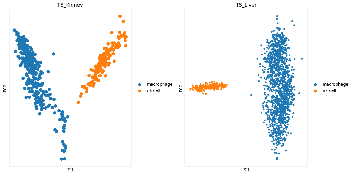
In this example, you will use the callback argument to perform a PCA on the selected cell types and visualize the results.

graph = build_collection_mapper_workflow_graph(
    soma_collection_uri=SOMA_COLLECTION_URI,
    experiment_names=["TS_Kidney", "TS_Liver"],
    measurement_name="RNA",
    X_layer_name="data",
    obs_query_string="cell_ontology_class in ['macrophage', 'nk cell']",
    var_query_string="highly_variable == True",
    obs_attrs=["cell_id", "cell_ontology_class"],
    var_attrs=["gene_symbol", "means", "highly_variable"],
    callback=sc.pp.pca,
    args_dict={"copy": True},
)

graph.visualize()

[2024-07-18 19:40:42,184] [mapper] [build_collection_mapper_workflow_graph] [INFO] Retrieving SOMA Experiment URIs from SOMACollection tiledb://tiledb-inc/soma-exps-tabula-sapiens-by-tissue
[2024-07-18 19:40:42,408] [mapper] [build_collection_mapper_workflow_graph] [INFO] Filtering SOMA Experiment URIs for specified names
[2024-07-18 19:40:42,410] [mapper] [build_collection_mapper_workflow_graph] [INFO] Retrieved 2 SOMA Experiment URIs
[2024-07-18 19:40:42,410] [mapper] [build_collection_mapper_workflow_graph] [INFO] Constructing task graph

graph.compute()
graph.wait()

Retrieve the results and note the presence of the new PCA items in the obsm, varm, and uns attributes of the AnnData objects.

results = graph.end_results_by_name()
results

{'TS_Kidney': AnnData object with n_obs × n_vars = 452 × 2435
     obs: 'cell_id', 'cell_ontology_class'
     var: 'gene_symbol', 'means', 'highly_variable'
     uns: 'pca'
     obsm: 'X_pca'
     varm: 'PCs',
 'TS_Liver': AnnData object with n_obs × n_vars = 1626 × 2435
     obs: 'cell_id', 'cell_ontology_class'
     var: 'gene_symbol', 'means', 'highly_variable'
     uns: 'pca'
     obsm: 'X_pca'
     varm: 'PCs'}

Now you can visualize the PCA results for each experiment.

fig, axs = plt.subplots(1, len(results), figsize=(12, 6))

for i, (name, adat) in enumerate(results.items()):
    sc.pl.pca(adat, ax=axs[i], show=False, color="cell_ontology_class")
    axs[i].set_title(name)

plt.tight_layout()
plt.show()

Figure 1

Conclusion

The SOMA Experiment Collection Mapper UDF is a versatile and powerful tool that enables efficient and scalable data processing across multiple SOMA experiments.