Access Spatial Data

Learn how to access the spatial data components of a SOMA Experiment.

TileDB-SOMA supports spatial omics data, such as those generated by 10X Visium. SOMA experiments created from these spatial datasets include extra elements beyond typical single-cell experiments, such as high-resolution tissue images and spatial coordinates for each measurement location. This tutorial guides you through understanding these new spatial components and shows how to access them using TileDB-SOMA’s API. You’ll learn how to do the following:

• Open a TileDB-SOMA experiment with spatial data.
• Navigate the experiment’s spatial components, including scenes, images, and spatial dataframes.
• Load image data for visualization.
• Access spatial location data using bounding boxes.

Prerequisites

While you can run this tutorial locally, note that this tutorial relies on remote resources to run correctly.

You must create a REST API token and create an environment variable named $TILEDB_REST_TOKEN set to the value of your generated token.

However, this is not necessary when running this notebook inside of a TileDB workspace where the API token is automatically generated and configured for you.

Setup

Load the necessary packages. Import tiledbsoma to interact with SOMA data, scanpy for some data visualization, and matplotlib for displaying images and plots.

Python

import scanpy as sc
import tiledbsoma
import tiledbsoma.io
from matplotlib import patches as mplp
from matplotlib import pyplot as plt
from matplotlib.collections import PatchCollection

tiledbsoma.show_package_versions()

Configure the notebook to display images in jpeg format, which keeps the size of the rendered notebook smaller.

Python

import matplotlib_inline.backend_inline

matplotlib_inline.backend_inline.set_matplotlib_formats("jpeg")

Dataset

The dataset used here is a spatial gene expression dataset of a mouse brain coronal section (FFPE), generated by 10X Genomics’ Visium CytAssist platform. To view the raw data, visit 10x Genomics. This data has been processed with Space Ranger and ingested into TileDB-SOMA. You can find it on TileDB.

Tip

Visit the Spatial Data Ingestion tutorial for information on how to create a SOMA experiment from a spatial dataset.

Python

EXPERIMENT_URI = "tiledb://tiledb-inc/CytAssist_FFPE_Mouse_Brain_Rep2"

Navigate spatial components

Open the SOMA experiment in read mode. This action loads the experiment’s structure into memory. Note that the actual data is not loaded at this point, as it is only a pointer to the data on disk.

Python

exp = tiledbsoma.Experiment.open(EXPERIMENT_URI)
exp

<Experiment 'tiledb://tiledb-inc/CytAssist_FFPE_Mouse_Brain_Rep2' (open for 'r') (4 items)
    'ms': 'tiledb://TileDB-Inc/84fb4d8b-017d-4692-a356-267c0175305d' (unopened)
    'obs': 'tiledb://TileDB-Inc/45857df6-dd60-4d48-931c-878830339b71' (unopened)
    'obs_spatial_presence': 'tiledb://TileDB-Inc/2a909b4c-135e-4faf-a945-2d7029d82af1' (unopened)
    'spatial': 'tiledb://TileDB-Inc/58fab955-1470-483e-8c79-ae55d201382b' (unopened)>

As you can see in the output, the SOMA experiment consists of three top-level attributes, ms (measurements), obs (observation annotations), and spatial. The ms and obs attributes are common to all SOMA experiments, while the spatial attribute is specific to spatial experiments and stores all spatial data associated with the experiment.

It’s worth noting that even within a spatial SOMA experiment, you can access and query the non-spatial elements, such as the obs and ms collections, by using the same methods and APIs as with typical non-spatial SOMA experiments. This means that you can use familiar filtering, slicing, and data loading techniques with TileDB-SOMA for single-cell data, offering a consistent workflow, whether you’re working with spatial or non-spatial data components.

For example, read the var data from the SOMA Experiment as a pandas.DataFrame:

Python

MEASUREMENT_NAME = "RNA"

var_df = (
    exp.ms[MEASUREMENT_NAME]
    .var.read(column_names=["soma_joinid", "var_id", "gene_ids"])
    .concat()
    .to_pandas()
)
var_df

	soma_joinid	var_id	gene_ids
0	0	Xkr4	ENSMUSG00000051951
1	1	Rp1	ENSMUSG00000025900
2	2	Sox17	ENSMUSG00000025902
3	3	Lypla1	ENSMUSG00000025903
4	4	Tcea1	ENSMUSG00000033813
...	...	...	...
19460	19460	Zfy2	ENSMUSG00000000103
19461	19461	Sry	ENSMUSG00000069036
19462	19462	Gm4064	ENSMUSG00000102053
19463	19463	Gm3376	ENSMUSG00000096520
19464	19464	Gm20830	ENSMUSG00000096686

19465 rows × 3 columns

Load the non-spatial elements into memory as a standard AnnData object.

Python

adata = tiledbsoma.io.to_anndata(
    experiment=exp,
    measurement_name=MEASUREMENT_NAME,
    X_layer_name="data",
)

adata

AnnData object with n_obs × n_vars = 2235 × 19465
    var: 'gene_ids', 'feature_types', 'genome'

Spatial components

The spatial collection organizes the spatial data elements. This collection stores all spatial information associated with your experiment.

Python

exp.spatial

<Collection 'tiledb://TileDB-Inc/58fab955-1470-483e-8c79-ae55d201382b' (open for 'r') (1 item)
    'scene0': 'tiledb://TileDB-Inc/8aec3f0f-4ec1-40cf-a180-a1ba8a80f49e' (unopened)>

Scenes

Inside the spatial collection, you can find one or more Scene objects. A scene represents a distinct view or a physical section of the sample. This particular dataset has a single scene called scene0.

Python

scene = exp.spatial["scene0"]
scene

<Scene 'tiledb://TileDB-Inc/8aec3f0f-4ec1-40cf-a180-a1ba8a80f49e' (open for 'r') (3 items)
    'img': 'tiledb://TileDB-Inc/fbf2da75-dbcf-4e12-9e0c-2e6516a58bf0' (unopened)
    'obsl': 'tiledb://TileDB-Inc/47b25792-b016-4157-8cf2-ee534b3a2fad' (unopened)
    'varl': 'tiledb://TileDB-Inc/ddd4ae97-9ef3-4579-a0e4-3fbb821134a3' (unopened)>

Each Scene includes a coordinate space shared by all its members.

Python

scene.coordinate_space

CoordinateSpace(axes=(Axis(name='x', unit='pixels'), Axis(name='y', unit='pixels')))

A Scene has three key SOMA collections:

• img: This collection stores image data, such as the high- and low-resolution slide images of the tissue sample.
• obsl: This collection stores the obs-indexed location data. In this case, it has a PointCloudDataFrame called loc, holding the Visium spot locations and sizes.
• varl: This collection stores the var-indexed location data. In this example, the collection is empty because Visium datasets don’t include spatial feature data.

Images

Inside the img collection, you will find one or more MultiscaleImage objects.

Python

scene.img

<Collection 'tiledb://TileDB-Inc/fbf2da75-dbcf-4e12-9e0c-2e6516a58bf0' (open for 'r') (1 item)
    'tissue': 'tiledb://TileDB-Inc/bec86aa9-08a7-4a34-9887-8e7e2a117845' (unopened)>

In this example, a single MultiscaleImage image named “tissue” exists.

Python

tissue_image = scene.img["tissue"]
tissue_image

<MultiscaleImage 'tiledb://TileDB-Inc/bec86aa9-08a7-4a34-9887-8e7e2a117845' (open for 'r')>

This object has a pyramid of images at different resolutions, which supports efficient loading of each zoom level.

The coordinate_space property of the MultiscaleImage has the pixel coordinate space of the image.

Python

tissue_image.coordinate_space

CoordinateSpace(axes=(Axis(name='x', unit='pixels'), Axis(name='y', unit='pixels')))

Use the level_count property to see the number of levels in the MultiscaleImage.

Python

tissue_image.level_count

2

Examine the metadata for each image resolution level in the tissue collection.

Python

tissue_image.levels()

{'hires': ('tiledb://TileDB-Inc/2d8e4e5c-83ee-4b8f-aedf-7dde1988490f',
  (2000, 1692, 3)),
 'lowres': ('tiledb://TileDB-Inc/6c0db493-6a7f-4078-ad28-ed11b87cd572',
  (600, 508, 3))}

Each image is a DenseNDArray with dimensions corresponding to the image’s width, height, and color channels (RGB).

Python

tissue_image["hires"].schema

soma_dim_0: int64 not null
soma_dim_1: int64 not null
soma_dim_2: int64 not null
soma_data: uint8 not null

You can use the DenseNDArray’s read method to load the image data. This next snippet shows how to load the low-resolution image data and store the results as a NumPy array with shape (height, width, channels).

Python

im = tissue_image["lowres"].read().to_numpy()
im.shape

(600, 508, 3)

Now, visualize the low-resolution image with matplotlib.

Python

fig, ax = plt.subplots()
ax.imshow(im, cmap="gray")
plt.show()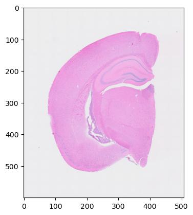

Spatial Dataframe

The obsl collection has a PointCloudDataFrame called loc, which holds the spatial coordinates for each spot in the experiment.

Python

scene.obsl["loc"]

<PointCloudDataFrame 'tiledb://TileDB-Inc/fadabf5c-2bf1-4d0b-a6b2-e124f89f3461' (open for 'r')>

Just like with the MultiscaleImage, you can access the coordinate_space property of the PointCloudDataFrame to see the coordinate space of the point cloud.

Python

scene.obsl["loc"].coordinate_space

CoordinateSpace(axes=(Axis(name='x', unit='pixels'), Axis(name='y', unit='pixels')))

This spatial dataframe has a key soma_joinid that maps to the obs array in the root of the SOMA experiment and the x and y coordinates of each spot. Read the data from the loc dataframe into memory.

Python

spots = scene.obsl["loc"].read().concat().to_pandas()
spots

	x	y	soma_joinid	in_tissue	array_row	array_col	spot_diameter_fullres
0	4008	11916	688	1	41	23	255.860716
1	3698	13834	1258	1	35	21	255.860716
2	3853	12875	462	1	38	22	255.860716
3	3871	13511	807	1	36	22	255.860716
4	4026	12552	1903	1	39	23	255.860716
...	...	...	...	...	...	...	...
2230	19018	18796	261	1	18	104	255.860716
2231	19192	18472	64	1	19	105	255.860716
2232	18535	21037	377	1	11	101	255.860716
2233	18554	21672	1728	1	9	101	255.860716
2234	18708	20713	768	1	12	102	255.860716

2235 rows × 7 columns

You can use the read_spatial_region method to perform a spatial query and retrieve the spots within a defined bounding box:

Python

scene.obsl["loc"].read_spatial_region(
    region=[3000, 3000, 10000, 10000]
).data.concat().to_pandas()

	x	y	soma_joinid	in_tissue	array_row	array_col	spot_diameter_fullres
0	5048	9977	2012	1	47	29	255.860716
1	5222	9654	1399	1	48	30	255.860716
2	5395	9331	1069	1	49	31	255.860716
3	5414	9967	1576	1	47	31	255.860716
4	5568	9008	1185	1	50	32	255.860716
...	...	...	...	...	...	...	...
119	9934	8244	823	1	52	56	255.860716
120	9971	9515	640	1	48	56	255.860716
121	8318	9246	2234	1	49	47	255.860716
122	8702	9871	2103	1	47	49	255.860716
123	9953	8880	2065	1	50	56	255.860716

124 rows × 7 columns

Finally, visualize the tissue spots with matplotlib.

Python

radius = scene.obsl["loc"].metadata["soma_geometry"]

spot_patches = PatchCollection(
    [
        mplp.Circle((row["x"], row["y"]), radius=radius, color="b")
        for _, row in spots.iterrows()
    ]
)

fig, ax = plt.subplots()
ax.set_xlim((0, spots["x"].max()))
ax.set_ylim((0, spots["y"].max()))
ax.invert_yaxis()
ax.add_collection(spot_patches)
plt.show()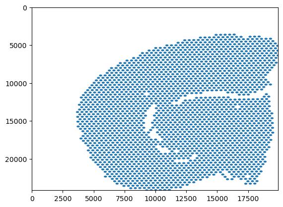

Summary

This tutorial covered basic methods for accessing spatial data within a SOMA experiment. This should give a solid foundation for building more complex spatial access patterns with TileDB-SOMA.