Population Genomics Data Model
This section describes the data models used in TileDB-VCF for the data array and variant statistics arrays. The detailed TileDB-VCF format is covered in the Storage Format Spec section, whereas the Key Concepts section describes important background information in the internal mechanics of TileDB-VCF.
Data array
Population variant data can be efficiently represented using a 3D sparse array. The dimensions of a TileDB-VCF dataset 3D array are always the following:
chromosome(also known ascontig)position- the start position of the variantsample- the sample name
For each sample, imagine a 2D plane where the vertical axis is the contig and the horizontal axis is the genomic position. Every variant can be represented as a range within this plane; it can be unary (i.e., a SNP) or it can be a longer range (e.g., INDEL or CNV). Each sample is then indexed by a third dimension, which is unbounded to accommodate populations of any size. The figure below shows an example for one sample, with several variants distributed across contigs chr1, chr2 and chr3.
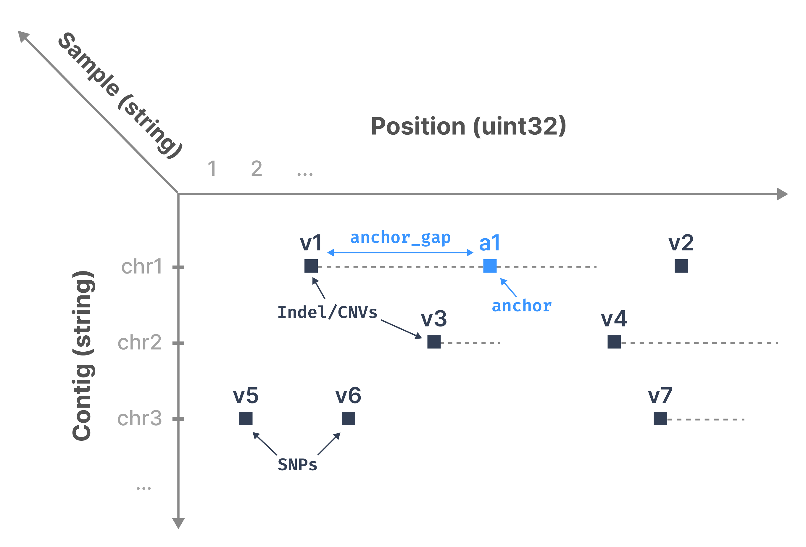
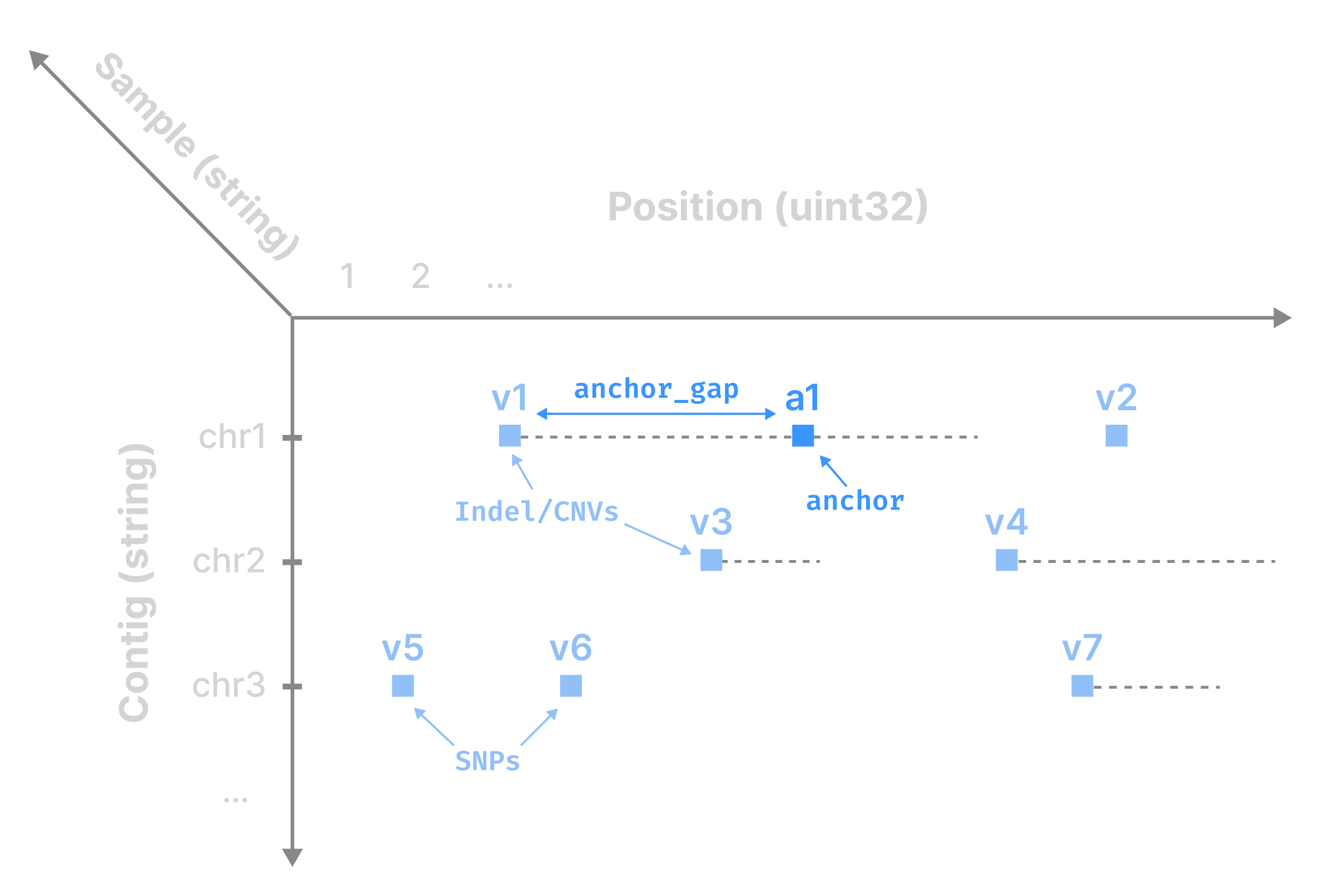
TileDB-VCF represents the start position of each range as a non-empty cell in a sparse array (all vi squares in the above figure). In each of those array cells, TileDB-VCF stores the end position of each cell (to create a range) along with all other fields in the corresponding single-sample VCF files for each variant (e.g., REF, ALT, etc.). Therefore, for every sample, variants are mapped to 2D non-empty sparse array cells.
To facilitate rapid retrieval of interval intersections, TileDB-VCF also injects anchors (a1 in the above figure) to breakup long ranges. Specifically, TileDB-VCF creates a new non-empty cell every anchor_gap bases from the start of the range (where anchor_gap is a user-defined parameter), which is identical to the range cell, except that (1) it has a new start coordinate and (2) it stores the real start position in an attribute.
Note that regardless of the number of samples, TileDB-VCF does not inject any additional information other than that of the anchors, which is user configurable and negligible for real datasets. In other words, this solution leads to linear storage in the number of samples, thus being scalable.
The typical access pattern used for variant data involves one or more rectangles covering a set of genomic ranges across one or more samples. The figure below demonstrates the user’s query as a dark blue rectangle. Observe that the results are highlighted in light blue (v1, v2, v4, v7). However, the rectangle misses v1 (i.e., the case where an Indel/CNV range intersects the query rectangle, but the start position is outside the rectangle).
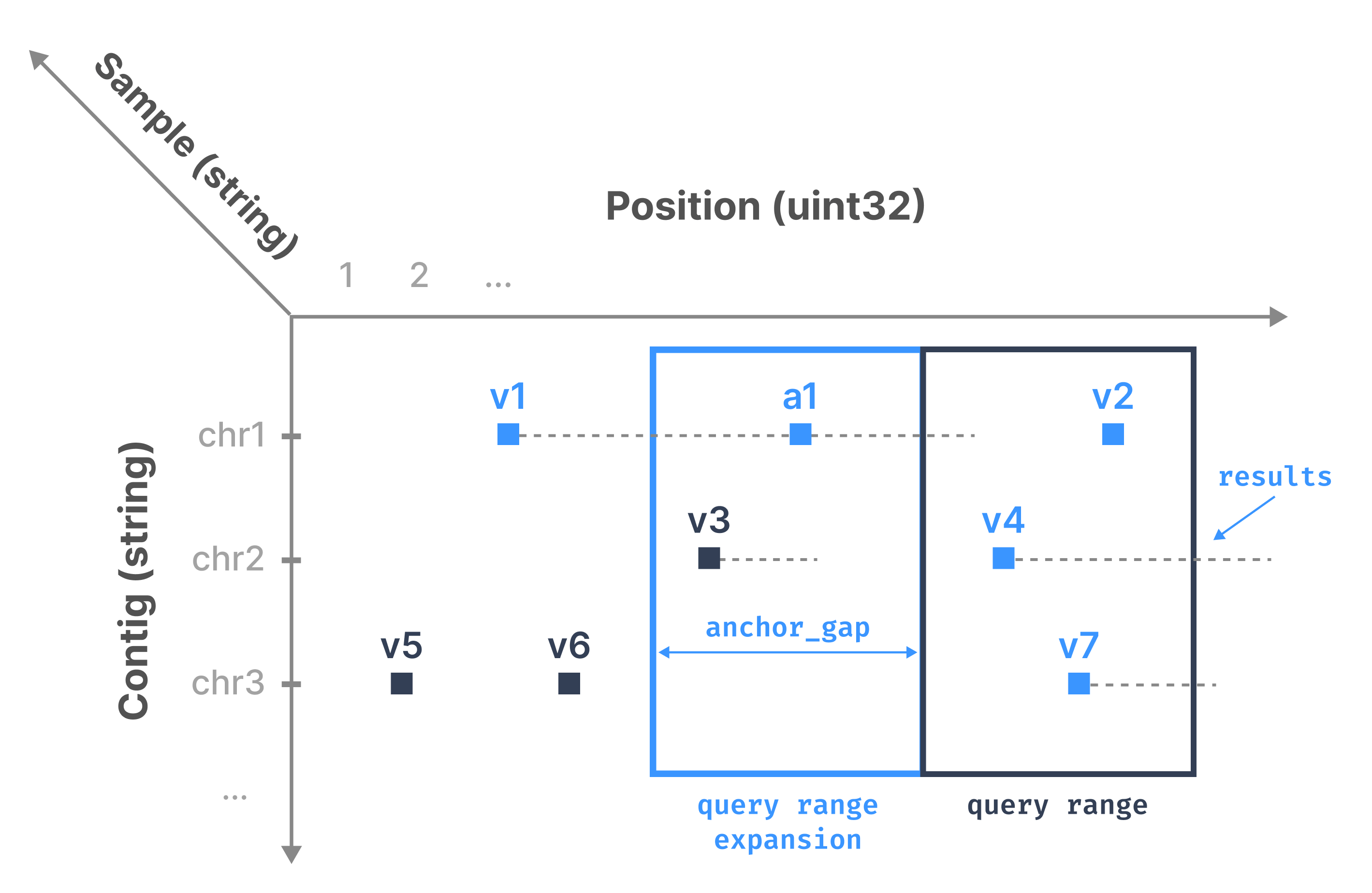
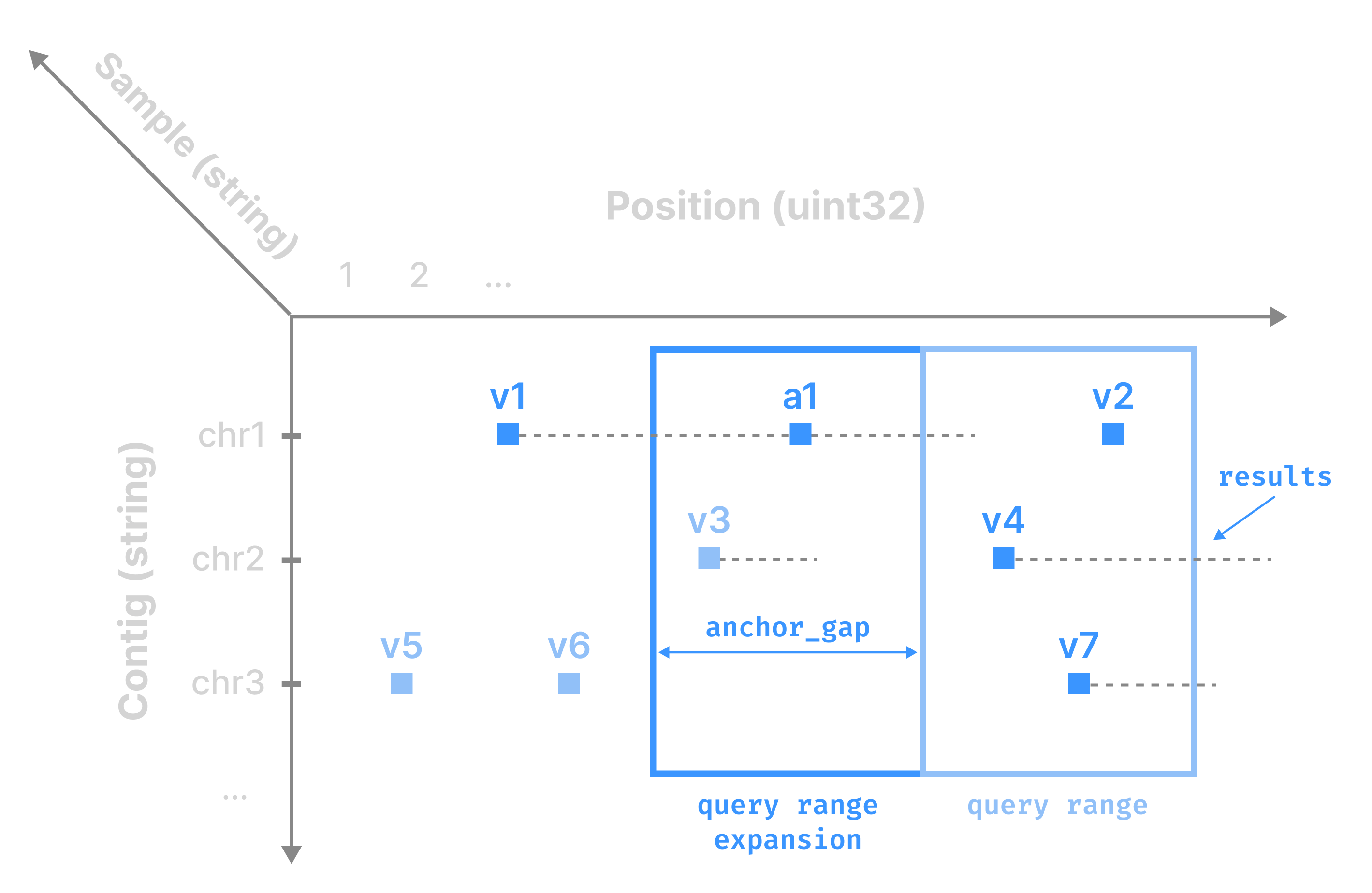
This is the motivation behind anchors. TileDB-VCF expands the user’s query range on the left by anchor_gap. It then reports as results the cells that are included in the expanded query if their end position (stored in an attribute) comes after the query range start endpoint. In the example above, TileDB-VCF retrieves anchor a1 and Indel/CNV v3. It reports v1 as a result (as it can be extracted directly from anchor a1), but filters out v3.
Quite often, the analyses require data retrieval based on numerous query ranges (up to the order of millions), which must be submitted simultaneously. TileDB-VCF leverages the highly optimized multi-range subarray functionality.
Variant statistics arrays
The TileDB-VCF data model includes arrays to hold a variety of summary statistics. Visit Key Concepts Variant Statistics for more background on the lifecycle of these statistics, including how they are ingested, stored, aggregated, appended, consolidated, and deleted. The data model for each of the variant statistics arrays is described in this section.
Variant stats
The variant_stats array holds data used to compute internal allele frequency (IAF), specifically the allele count for every chrom-pos-allele in the dataset.
The data is stored in a 2D sparse array with the following dimensions:
contig- the chromosome orCHROMfrom the VCF filepos- the start position of the variant
This array is primarily accessed with genomic regions (for example, chr19:44905804-44909392), which maps to a contig value and a range of pos values. The array allows cell multiplicities (i.e. duplicate coordinate values), which means any [contig, pos] coordinate value can contain multiple cells in the array, where each cell contains a portion of the total result for that coordinate. Allowing duplicate coordinate values provides a scalable method for adding data to the array. TileDB-VCF provides a read API that aggregates the values appropriately, as shown in the variant statistics tutorial.
Allele count
The allele_count array holds counts of unique chrom-pos-ref-alt variants in the dataset. The data model is very similar to the variant_stats array.
The data is stored in a 2D sparse array with the following dimensions:
contig- the chromosome orCHROMfrom the VCF filepos- the start position of the variant
The array is primarily accessed with genomic regions (for example, chr19:44905804-44909392), which maps to a contig value and a range of pos values. The array allows cell multiplicities (i.e. duplicate coordinate values), which means any [contig, pos] coordinate value may contain multiple cells in the array, where each cell contains a portion of the total result for that coordinate. Allowing duplicate coordinate values provides a scalable method for adding data to the array. TileDB-VCF provides a read API that aggregates the values appropriately, as shown in the variant statistics tutorial.
Sample stats
The sample_stats array holds variant summary statistics for each sample, similar to Hail’s sample_qc and bcftools stats.
The data is stored in a 1D sparse array with a single dimension named sample, containing the sample name.
The array allows cell multiplicities (i.e. duplicate coordinate values), which means a sample may contain multiple cells in the array, with each cell containing a portion of the total statistics for that sample. TileDB-VCF provides a read API that aggregates the values appropriately.