Manage Coordinate Spaces

Learn how to manage spatial coordinates in TileDB-SOMA.

This tutorial will guide you through the fundamental concepts of coordinate spaces and coordinate transformations within TileDB-SOMA. These concepts are essential for working with any of the spatial SOMA objects, including MultiscaleImage, PointCloudDataFrame, and GeometryDataFrame.

By the end of this tutorial, you’ll understand how to:

• Define a coordinate space.
• Associate coordinate spaces with spatial objects.
• Create and use coordinate transformations.

Setup

First, import the necessary libraries:

Python

import tempfile
from typing import Optional, Sequence

import pyarrow as pa
import pyarrow.compute as pc
import tiledbsoma
import tiledbsoma.io
import tiledbsoma.io.spatial
from matplotlib import patches as mplp
from matplotlib import pyplot as plt
from matplotlib.collections import PatchCollection

tiledbsoma.show_package_versions()

Define the TileDB Cloud SaaS URI for a spatial SOMA experiment containing a 10X Visium generated from a mouse brain coronal section.

Python

EXPERIMENT_URI = "tiledb://tiledb-inc/CytAssist_FFPE_Mouse_Brain_Rep2"

Open the experiment in read mode:

Python

exp = tiledbsoma.Experiment.open(EXPERIMENT_URI)
scene = exp.spatial["scene0"]
scene

<Scene 'tiledb://TileDB-Inc/8aec3f0f-4ec1-40cf-a180-a1ba8a80f49e' (open for 'r') (3 items)
    'img': 'tiledb://TileDB-Inc/fbf2da75-dbcf-4e12-9e0c-2e6516a58bf0' (unopened)
    'obsl': 'tiledb://TileDB-Inc/47b25792-b016-4157-8cf2-ee534b3a2fad' (unopened)
    'varl': 'tiledb://TileDB-Inc/ddd4ae97-9ef3-4579-a0e4-3fbb821134a3' (unopened)>

Create and Access Coordinate Spaces

A coordinate space defines the frame of reference for your spatial data. Think of it as the “grid” or “axes” upon which your data points, images, or shapes are positioned. Each coordinate space has a set of named axes, and each axis has a defined unit of measurement. This information is stored as metadata and is distinct from any coordinates for data located on the coordinate system.

This section demonstrates how to create coordinate spaces in TileDB-SOMA.

The most common scenario is a 2D space, often representing the X and Y dimensions of an image or tissue section. A 2D space with axes named “x” and “y”, using “pixels” as the unit, can be created as follows:

Python

coords2d = tiledbsoma.CoordinateSpace(
    axes=[
        tiledbsoma.Axis(name="x", unit="pixels"),
        tiledbsoma.Axis(name="y", unit="pixels"),
    ]
)

coords2d

CoordinateSpace(axes=(Axis(name='x', unit='pixels'), Axis(name='y', unit='pixels')))

The coordinate space defines the meaning of the coordinates, but it doesn’t store the coordinate values themselves. The actual values are stored within the spatial objects like PointCloudDataFrame, GeometryDataFrame, or DenseNDArray within a MultiscaleImage.

The coordinate spaces are stored as metadata on the underlying TileDB groups and arrays. They are accessible via the coordinate_space attribute of any SOMA spatial object. The coordinate space of the scene in the experiment can be accessed as follows:

Python

scene.coordinate_space

CoordinateSpace(axes=(Axis(name='x', unit='pixels'), Axis(name='y', unit='pixels')))

Create Spatial Objects with Coordinate Spaces

Now that you know how to define coordinate spaces, this section shows how to associate them with the actual spatial data objects in TileDB-SOMA. You will primarily use the PointCloudDataFrame for these examples, as it’s the most straightforward to visualize, but the same principles apply to GeometryDataFrame and MultiscaleImage.

A small PointCloudDataFrame can be created to represent a few points in a 2D space. The coords2d object defined earlier (with “x” and “y” axes in pixels) will be used.

Python

tbl = pa.Table.from_pydict(
    {
        "x": pa.array([10, 20, 15]),
        "y": pa.array([5, 5, 12]),
        "intensity": pa.array([0.8, 0.2, 0.9]),
        "soma_joinid": pa.array([0, 1, 2]),
    }
)


with tiledbsoma.PointCloudDataFrame.create(
    uri=tempfile.mkdtemp(prefix="tiledb-soma-pcdf-"),
    schema=tbl.schema,
    coordinate_space=coords2d,
    domain=[[0, 20], [0, 20], [0, 2]],
) as pcdf:
    pcdf.write(tbl)

pcdf

<PointCloudDataFrame '/tmp/tiledb-soma-pcdf-qa37umnb' (CLOSED for 'w')>

Now open the PointCloudDataFrame and access the coordinate space information:

Python

with tiledbsoma.PointCloudDataFrame.open(pcdf.uri, mode="r") as pcdf:
    print(pcdf.coordinate_space)

CoordinateSpace(axes=(Axis(name='x', unit='pixels'), Axis(name='y', unit='pixels')))

The output confirms that the PointCloudDataFrame is associated with the 2D coordinate space defined earlier.

Apply Coordinate Transforms

Coordinate transforms are essential for relating data that exists in different coordinate spaces. A coordinate transform defines a mapping from one coordinate space to another. In TileDB-SOMA, transforms are applied to data when you read it. They are not stored as part of the data itself. This allows the data to be written on a native coordinate system but read in other coordinate systems.

To prove this, you will project both the Visium spots and images to a common coordinate space. First, retrieve the coordinate space of from the SOMAScene accessed earlier:

Python

scene.coordinate_space

CoordinateSpace(axes=(Axis(name='x', unit='pixels'), Axis(name='y', unit='pixels')))

Retrieve the coordinate transform from the scene’s coordinate space to the PointCloudDataFrame’s coordinate space.

Python

scene.get_transform_to_point_cloud_dataframe("loc")

<IdentityTransform
  input axes: ('x', 'y')
  output axes: ('x', 'y')>

This returns an IdentityTransform, because the PointCloudDataFrame’s coordinate space is the same as the scene’s coordinate space.

Next retrieve the coordinate transform from the scene’s coordinate space to the MultiscaleImage’s coordinate space.

Python

fullres_to_image = scene.get_transform_to_multiscale_image("tissue")
fullres_to_image

<ScaleTransform
  input axes: ('x', 'y')
  output axes: ('x', 'y')
  scales: [0.07127211 0.07127076]>

Here, TileDB-SOMA returns a ScaleTransform, because the MultiscaleImage’s coordinate space was downsampled relative to the full resolution image used to map the Visium spots.

You can use these transforms to project the Visium spots onto a region of interest in the high-resolution image. This will require you to do the following:

• Read the region from the high-resolution level of the MultiScaleImage.
• Read the same region from the PointCloudDataFrame storing the spot locations.
• Use the transformation from the MultiscaleImage to scale align the spot locations with the image.

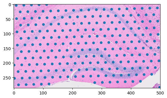
First, specify the region of interest that encompasses the hippocampus.

Python

x_min, x_max = (12000, 19000)
y_min, y_max = (7500, 11500)

hippo_region = [x_min, y_min, x_max, y_max]

Use the bounding box to perform a spatial query on the loc dataframe to get the spots within the region of interest.

Python

region_spots = (
    scene.obsl["loc"].read_spatial_region(region=hippo_region).data.concat().to_pandas()
)

region_spots

	x	y	soma_joinid	in_tissue	array_row	array_col	spot_diameter_fullres
0	12108	7544	459	1	54	68	255.860716
1	12126	8180	220	1	52	68	255.860716
2	12145	8816	875	1	50	68	255.860716
3	12164	9452	729	1	48	68	255.860716
4	12182	10087	2072	1	46	68	255.860716
...	...	...	...	...	...	...	...
223	18932	9572	290	1	47	105	255.860716
224	18950	10208	285	1	45	105	255.860716
225	18777	10531	1569	1	44	104	255.860716
226	18988	11479	102	1	41	105	255.860716
227	18604	10854	2102	1	43	103	255.860716

228 rows × 7 columns

Now, use the read_spatial_region() method to load only the part of the image that has the hippocampus. When you pass the ScaleTransform object to the region_transform argument it automatically scales the region selected to the downsampled resolution.

Python

hires_read = scene.img["tissue"].read_spatial_region(
    level=0, region=hippo_region, region_transform=fullres_to_image
)
hires_read

SpatialRead(data=<pyarrow.Tensor>
type: uint8
shape: (287, 501, 3)
strides: (1503, 3, 1), data_coordinate_space=CoordinateSpace(axes=(Axis(name='x', unit='pixels'), Axis(name='y', unit='pixels'))), output_coordinate_space=CoordinateSpace(axes=(Axis(name='x', unit=None), Axis(name='y', unit=None))), coordinate_transform=<AffineTransform
  input axes: ('x', 'y')
  output axes: ('x', 'y')
  augmented matrix:
    [[1.40307329e+01 0.00000000e+00 1.19962766e+04]
     [0.00000000e+00 1.40310000e+01 7.49255400e+03]
     [0.00000000e+00 0.00000000e+00 1.00000000e+00]]>)

This returns a SpatialRead object that includes both the image data and the coordinate transform that scales and translates the returned data to the original coordinate space you queried. You can use the inverse of this transformation to convert the spot data into the coordinate space of the image data. Underneath the hood, the transforms are accessible directly as matrices:

Python

spot_to_hires_matrix = (
    hires_read.coordinate_transform.inverse_transform().augmented_matrix
)
spot_to_hires_matrix

array([[ 7.12721146e-02,  0.00000000e+00, -8.55000000e+02],
       [ 0.00000000e+00,  7.12707576e-02, -5.34000000e+02],
       [ 0.00000000e+00,  0.00000000e+00,  1.00000000e+00]])

You can use this matrix to manually project the data from the spot dataframe to the hires image’s resolution.

Python

scale_x = spot_to_hires_matrix[0, 0]
scale_y = spot_to_hires_matrix[1, 1]
offset_x = spot_to_hires_matrix[0, 2]
offset_y = spot_to_hires_matrix[1, 2]

And now, you can plot the spots and image data together.

Python

radius = scene.obsl["loc"].metadata["soma_geometry"]
spot_patches = PatchCollection(
    [
        mplp.Ellipse(
            (scale_x * row["x"] + offset_x, scale_y * row["y"] + offset_y),
            width=radius * scale_x,
            height=radius * scale_y,
            fill=False,
            alpha=0.8,
        )
        for _, row in region_spots.iterrows()
    ]
)

fig, ax = plt.subplots()
ax.imshow(hires_read.data)
ax.add_collection(spot_patches)

plt.show()