1. Structure
  2. Life Sciences
  3. Single-cell
  4. Tutorials
  5. Distributed Compute
  • Home
  • What is TileDB?
  • Get Started
  • Explore Content
  • Accounts
    • Individual Accounts
      • Apply for the Free Tier
      • Profile
        • Overview
        • Cloud Credentials
        • Storage Paths
        • REST API Tokens
        • Credits
    • Organization Admins
      • Create an Organization
      • Profile
        • Overview
        • Members
        • Cloud Credentials
        • Storage Paths
        • Billing
      • API Tokens
    • Organization Members
      • Organization Invitations
      • Profile
        • Overview
        • Members
        • Cloud Credentials
        • Storage Paths
        • Billing
      • API Tokens
  • Catalog
    • Introduction
    • Data
      • Arrays
      • Tables
      • Single-Cell (SOMA)
      • Genomics (VCF)
      • Biomedical Imaging
      • Vector Search
      • Files
    • Code
      • Notebooks
      • Dashboards
      • User-Defined Functions
      • Task Graphs
      • ML Models
    • Groups
    • Marketplace
    • Search
  • Collaborate
    • Introduction
    • Organizations
    • Access Control
      • Introduction
      • Share Assets
      • Asset Permissions
      • Public Assets
    • Logging
    • Marketplace
  • Analyze
    • Introduction
    • Slice Data
    • Multi-Region Redirection
    • Notebooks
      • Launch a Notebook
      • Usage
      • Widgets
      • Notebook Image Dependencies
    • Dashboards
      • Dashboards
      • Streamlit
    • Preview
    • User-Defined Functions
    • Task Graphs
    • Serverless SQL
    • Monitor
      • Task Log
      • Task Graph Log
  • Scale
    • Introduction
    • Task Graphs
    • API Usage
  • Structure
    • Why Structure Is Important
    • Arrays
      • Introduction
      • Quickstart
      • Foundation
        • Array Data Model
        • Key Concepts
          • Storage
            • Arrays
            • Dimensions
            • Attributes
            • Cells
            • Domain
            • Tiles
            • Data Layout
            • Compression
            • Encryption
            • Tile Filters
            • Array Schema
            • Schema Evolution
            • Fragments
            • Fragment Metadata
            • Commits
            • Indexing
            • Array Metadata
            • Datetimes
            • Groups
            • Object Stores
          • Compute
            • Writes
            • Deletions
            • Consolidation
            • Vacuuming
            • Time Traveling
            • Reads
            • Query Conditions
            • Aggregates
            • User-Defined Functions
            • Distributed Compute
            • Concurrency
            • Parallelism
        • Storage Format Spec
      • Tutorials
        • Basics
          • Basic Dense Array
          • Basic Sparse Array
          • Array Metadata
          • Compression
          • Encryption
          • Data Layout
          • Tile Filters
          • Datetimes
          • Multiple Attributes
          • Variable-Length Attributes
          • String Dimensions
          • Nullable Attributes
          • Multi-Range Reads
          • Query Conditions
          • Aggregates
          • Deletions
          • Catching Errors
          • Configuration
          • Basic S3 Example
          • Basic TileDB Cloud
          • fromDataFrame
          • Palmer Penguins
        • Advanced
          • Schema Evolution
          • Advanced Writes
            • Write at a Timestamp
            • Get Fragment Info
            • Consolidation
              • Fragments
              • Fragment List
              • Consolidation Plan
              • Commits
              • Fragment Metadata
              • Array Metadata
            • Vacuuming
              • Fragments
              • Commits
              • Fragment Metadata
              • Array Metadata
          • Advanced Reads
            • Get Fragment Info
            • Time Traveling
              • Introduction
              • Fragments
              • Array Metadata
              • Schema Evolution
          • Array Upgrade
          • Backends
            • Amazon S3
            • Azure Blob Storage
            • Google Cloud Storage
            • MinIO
            • Lustre
          • Virtual Filesystem
          • User-Defined Functions
          • Distributed Compute
          • Result Estimation
          • Incomplete Queries
        • Management
          • Array Schema
          • Groups
          • Object Management
        • Performance
          • Summary of Factors
          • Dense vs. Sparse
          • Dimensions vs. Attributes
          • Compression
          • Tiling and Data Layout
          • Tuning Writes
          • Tuning Reads
      • API Reference
    • Tables
      • Introduction
      • Quickstart
      • Foundation
        • Data Model
        • Key Concepts
          • Indexes
          • Columnar Storage
          • Compression
          • Data Manipulation
          • Optimize Tables
          • ACID
          • Serverless SQL
          • SQL Connectors
          • Dataframes
          • CSV Ingestion
      • Tutorials
        • Basics
          • Ingestion with SQL
          • CSV Ingestion
          • Basic S3 Example
          • Running Locally
        • Advanced
          • Scalable Ingestion
          • Scalable Queries
      • API Reference
    • AI & ML
      • Vector Search
        • Introduction
        • Quickstart
        • Foundation
          • Data Model
          • Key Concepts
            • Vector Search
            • Vector Databases
            • Algorithms
            • Distance Metrics
            • Updates
            • Deployment Methods
            • Architecture
            • Distributed Compute
          • Storage Format Spec
        • Tutorials
          • Basics
            • Ingestion & Querying
            • Updates
            • Deletions
            • Basic S3 Example
            • Running Locally
          • Advanced
            • Versioning
            • Time Traveling
            • Consolidation
            • Distributed Compute
            • RAG LLM
            • LLM Memory
            • File Search
            • Image Search
            • Protein Search
          • Performance
        • API Reference
      • ML Models
        • Introduction
        • Quickstart
        • Foundation
          • Basics
          • Storage
          • Cloud Execution
          • Why TileDB for Machine Learning
        • Tutorials
          • Ingestion
            • Data Ingestion
              • Dense Datasets
              • Sparse Datasets
            • ML Model Ingestion
          • Management
            • Array Schema
            • Machine Learning: Groups
            • Time Traveling
    • Life Sciences
      • Single-cell
        • Introduction
        • Quickstart
        • Foundation
          • Data Model
          • Key Concepts
            • Data Structures
            • Use of Apache Arrow
            • Join IDs
            • State Management
            • TileDB Cloud URIs
          • SOMA API Specification
        • Tutorials
          • Data Ingestion
          • Bulk Ingestion Tutorial
          • Data Access
          • Distributed Compute
          • Basic S3 Example
          • Multi-Experiment Queries
          • Appending Data to a SOMA Experiment
          • Add New Measurements
          • SQL Queries
          • Running Locally
          • Shapes in TileDB-SOMA
          • Drug Discovery App
        • Spatial
          • Introduction
          • Foundation
            • Spatial Data Model
            • Data Structures
          • Tutorials
            • Spatial Data Ingestion
            • Access Spatial Data
            • Manage Coordinate Spaces
        • API Reference
      • Population Genomics
        • Introduction
        • Quickstart
        • Foundation
          • Data Model
          • Key Concepts
            • The N+1 Problem
            • Architecture
            • Arrays
            • Ingestion
            • Reads
            • Variant Statistics
            • Annotations
            • User-Defined Functions
            • Tables and SQL
            • Distributed Compute
          • Storage Format Spec
        • Tutorials
          • Basics
            • Basic Ingestion
            • Basic Queries
            • Export to VCF
            • Add New Samples
            • Deleting Samples
            • Basic S3 Example
            • Basic TileDB Cloud
          • Advanced
            • Scalable Ingestion
            • Scalable Queries
            • Query Transforms
            • Handling Large Queries
            • Annotations
              • Finding Annotations
              • Embedded Annotations
              • External Annotations
              • Annotation VCFs
              • Ingesting Annotations
            • Variant Statistics
            • Tables and SQL
            • User-Defined Functions
            • Sample Metadata
            • Split VCF
          • Performance
        • API Reference
          • Command Line Interface
          • Python API
          • Cloud API
      • Biomedical Imaging
        • Introduction
        • Foundation
          • Data Model
          • Key Concepts
            • Arrays
            • Ingestion
            • Reads
            • User Defined Functions
          • Storage Format Spec
        • Quickstart
        • Tutorials
          • Basics
            • Ingestion
            • Read
              • OpenSlide
              • TileDB-Py
          • Advanced
            • Batched Ingestion
            • Chunked Ingestion
            • Machine Learning
              • PyTorch
            • Napari
    • Files
  • API Reference
  • Self-Hosting
    • Installation
    • Upgrades
    • Administrative Tasks
    • Image Customization
      • Customize User-Defined Function Images
      • AWS ECR Container Registry
      • Customize Jupyter Notebook Images
    • Single Sign-On
      • Configure Single Sign-On
      • OpenID Connect
      • Okta SCIM
      • Microsoft Entra
  • Glossary

On this page

  • Background
  • Objective
  • Setup
  • Base function
  • Serverless execution
  • Cloud server resources
  • UDF registration
  • Scaling with task graphs
  • Housekeeping
  1. Structure
  2. Life Sciences
  3. Single-cell
  4. Tutorials
  5. Distributed Compute

Use Distributed Compute with SOMA Datasets

life sciences
single cell (soma)
tutorials
python
scalable compute
Learn how to leverage TileDB Cloud’s serverless capabilities to perform distributed operations on single-cell data.
How to run this tutorial

You can run this tutorial only on TileDB Cloud. However, TileDB Cloud has a free tier. We strongly recommend that you sign up and run everything there, as that requires no installations or deployment.

TileDB Cloud’s serverless compute platform enables the execution of distributed compute tasks on single-cell datasets stored in TileDB-SOMA. This tutorial will cover how to:

  • Run an arbitrary function serverlessly on TileDB Cloud as a user-defined function (UDF).
  • Register a UDF with TileDB Cloud to simplify reuse and sharing.
  • Build and execute a task graph composed of multiple UDFs to perform a distributed operation.
  • Monitor the task graph’s progress.
  • Retrieve and visualize the task graph’s results.

Background

Serverless? UDFs? Task graphs? Oh my! Here’s a quick primer in case these concepts are new to you:

  • Serverless: Serverless computing allows you to run code without having to provision or manager servers. Instead, TileDB Cloud automatically spins-up a cloud-based server to run your code, and then shuts it down when the code is done executing. That way, you only pay for the time your code is running, and you don’t have to worry about managing servers.

  • UDFs: User-defined functions (UDFs) are custom functions that you can write in a variety of languages and run on TileDB Cloud.

  • Task graph: A task graph is a directed acyclic graph (DAG) that represents a series of tasks (i.e., UDFs) that need to be executed in a specific order that also accounts for dependencies between them.

Objective

Your mission is to build a reproducible workflow for calculating gene-wise summary statistics for a user-defined set of genes across a collection of single-cell RNA-seq experiments. In this tutorial, you will work with a collection of 24 tissue-specific datasets produced by the Tabula Sapiens consortium. Each of these datasets has been converted to a SOMA experiment and published as a collection on TileDB Cloud.

Setup

You will need to import the tiledbsoma and tiledb.cloud packages to run this tutorial, as well as a few other common libraries for data manipulation and visualization.

import matplotlib.pyplot as plt
import pyarrow as pa
import seaborn as sns
import tiledb.cloud
import tiledbsoma

Now define a couple constants that will be used throughout the tutorial.

  • NAMESPACE: The TileDB Cloud namespace that you are working in. You should update this with your own namespace.
  • SOCO_URI: The TileDB Cloud URI for accessing the collection of Tabula Sapiens SOMA experiments.
import os

NAMESPACE = os.environ["TILEDB_ACCOUNT"]
SOCO_URI = "tiledb://TileDB-Inc/soma-exps-tabula-sapiens-by-tissue"

Retrieve the list of SOMA experiments from the Tabula Sapiens collection.

with tiledbsoma.Collection.open(SOCO_URI) as soco:
    exp_uris = {k: v.uri for k, v in soco.items()}

exp_uris
{'TS_Vasculature': 'tiledb://TileDB-Inc/822014de-c530-49f7-959c-bb58753a884b',
 'TS_Bone_Marrow': 'tiledb://TileDB-Inc/66d75d38-88de-4178-81c6-0c3bc8285721',
 'TS_Lung': 'tiledb://TileDB-Inc/a5c53e63-ec4c-40b9-9806-b4e15cbc82d7',
 'TS_Lymph_Node': 'tiledb://TileDB-Inc/90240c79-8900-4b1d-aff4-478128cedf54',
 'TS_Fat': 'tiledb://TileDB-Inc/9ce37d99-d8b0-4ba3-8528-4db77072877a',
 'TS_Kidney': 'tiledb://TileDB-Inc/b499e2c3-6d5b-4cd3-9e98-48c19affc383',
 'TS_Large_Intestine': 'tiledb://TileDB-Inc/ac1dab32-2376-46be-a26d-c690f9f47496',
 'TS_Liver': 'tiledb://TileDB-Inc/ebc50605-fabe-4108-b8fb-68c2bfd4c7f1',
 'TS_Skin': 'tiledb://TileDB-Inc/6cee562f-07c6-45dc-a3c9-0d381770bec2',
 'TS_Heart': 'tiledb://TileDB-Inc/420f9b59-b701-4731-90aa-49b14d80d874',
 'TS_Muscle': 'tiledb://TileDB-Inc/27918566-d931-471a-b5db-111594fe77ac',
 'TS_Eye': 'tiledb://TileDB-Inc/ed7a9a8b-081c-467c-8fa3-2617eb31ad8b',
 'TS_Bladder': 'tiledb://TileDB-Inc/a07f527e-4b24-44c7-8cf6-fb304f6c74db',
 'TS_Pancreas': 'tiledb://TileDB-Inc/66718a75-dd5b-49e1-a362-0842dc88c872',
 'TS_Prostate': 'tiledb://TileDB-Inc/29c85217-180a-420a-83f9-33043e92d1c8',
 'TS_Uterus': 'tiledb://TileDB-Inc/1d02f4f1-6134-44d8-9875-043f969cc03a',
 'TS_Salivary_Gland': 'tiledb://TileDB-Inc/8177e51f-5b10-48dd-996f-29c30c0806de',
 'TS_Blood': 'tiledb://TileDB-Inc/7210bc54-923d-4e2b-a240-caf68e58cec8',
 'TS_Small_Intestine': 'tiledb://TileDB-Inc/427b8b25-cd8e-4d19-b1d8-ea59ae8598ca',
 'TS_Spleen': 'tiledb://TileDB-Inc/61bfa777-e550-4eeb-9262-4b8754b111ca',
 'TS_Thymus': 'tiledb://TileDB-Inc/0f209145-9b06-4792-83ed-e485eb00a7c7',
 'TS_Tongue': 'tiledb://TileDB-Inc/6136ee37-ee67-44ec-8c6c-80e74b44eb9d',
 'TS_Trachea': 'tiledb://TileDB-Inc/93f2bc52-9678-47e6-80cb-e8fa94c595b1',
 'TS_Mammary': 'tiledb://TileDB-Inc/302ec8df-27ef-4b44-8e73-171c6eb6cb44'}

Base function

The first step is to write the function that will calculate summary statistics for a given set of genes in a SOMA experiment. Then step-by-step you will see how to leverage TileDB Cloud’s functionality to run this function serverlessly and then in parallel across multiple experiments at once.

def soma_gene_stats(
    uri: str,
    *,
    measurement_name: str,
    X_layer_name: str,
    obs_query_string=None,
    var_query_string=None,
):
    import concurrent.futures

    import tiledbsoma
    import tiledbsoma.io

    obs_query = (
        tiledbsoma.AxisQuery(value_filter=obs_query_string)
        if obs_query_string is not None
        else None
    )
    var_query = (
        tiledbsoma.AxisQuery(value_filter=var_query_string)
        if var_query_string is not None
        else None
    )

    with tiledbsoma.Experiment.open(uri) as exp:
        with exp.axis_query(
            measurement_name=measurement_name,
            obs_query=obs_query,
            var_query=var_query,
        ) as query:
            with concurrent.futures.ThreadPoolExecutor() as executor:
                var_tbl = (
                    executor.submit(
                        query.var, column_names=["soma_joinid", "gene_symbol"]
                    )
                    .result()
                    .concat()
                )
                X_tbl = (
                    executor.submit(query.X, layer_name=X_layer_name)
                    .result()
                    .tables()
                    .concat()
                )

    return (
        X_tbl.group_by("soma_dim_1")
        .aggregate(
            [("soma_data", "mean"), ("soma_data", "stddev"), ("soma_data", "count")]
        )
        .join(var_tbl, keys=["soma_dim_1"], right_keys=["soma_joinid"])
    )

Now run it locally to verify that the function works as expected.

tbl = soma_gene_stats(
    uri=exp_uris["TS_Liver"],
    measurement_name="RNA",
    X_layer_name="data",
    # obs_query_string="n_genes > 1000",
    var_query_string="gene_symbol in ['CD19', 'CD3E', 'CD4', 'CD8A', 'CD14']",
)

tbl.to_pandas()
soma_dim_1 soma_data_mean soma_data_stddev soma_data_count gene_symbol
0 6745 2.689637 1.569328 161 CD8A
1 17012 2.220359 1.077917 2979 CD14
2 34045 3.391586 1.556160 1740 CD4
3 33468 1.899386 1.037067 178 CD3E
4 43535 3.891039 1.958365 22 CD19

Perfect! Now, you will see how to serverlessly execute this function on TileDB Cloud.

Serverless execution

TileDB Cloud’s serverless compute platform allows you to run any UDF on the cloud. In practice, this means the function’s code is serialized and shipped to a cloud-based server where it is executed before the results are returned to your session.

Just pass the callable function and its arguments to tiledb.cloud.udf.exec() to execute it on TileDB Cloud.

result = tiledb.cloud.udf.exec(
    soma_gene_stats,
    uri=exp_uris["TS_Liver"],
    measurement_name="RNA",
    X_layer_name="data",
    # obs_query_string="n_genes > 1000",
    var_query_string="gene_symbol in ['CD19', 'CD3E', 'CD4', 'CD8A', 'CD14']",
)

result.to_pandas()
soma_dim_1 soma_data_mean soma_data_stddev soma_data_count gene_symbol
0 6745 2.689637 1.569328 161 CD8A
1 17012 2.220359 1.077917 2979 CD14
2 34045 3.391586 1.556160 1740 CD4
3 33468 1.899386 1.037067 178 CD3E
4 43535 3.891039 1.958365 22 CD19

As expected, the results are the same as when you ran the function locally. However, this time a TileDB Cloud-based server performed the operation, rather than the machine running this notebook.

This serverless approach provides several immediate benefits:

  • Scalability: With very little effort, you can run any function on a server with more resources than your local machine.
  • Cost: You only pay for the time the function is running, rather than having to maintain a server that is always on or go through the hassle of spinning up and shutting down servers as needed.
  • Auditability: All serverless executions are logged and can be reviewed at any time. Visit https://cloud.tiledb.com/monitor/logs/tasks to see a list of all UDFs that have been executed, including the one you just ran.

Selecting the executed UDF’s entry in the TileDB Cloud Logs view will provide details about the UDF, including the function’s source code, how long it took to run, and the total cost of running it.

This information is also retrievable programmatically:

tiledb.cloud.last_udf_task()
{'access_cost': None,
 'activity': None,
 'array_metadata': None,
 'client_node_uuid': None,
 'cost': 1.93621963262558e-07,
 'cpu': 2,
 'description': None,
 'duration': 10134175951.0,
 'egress_cost': 1.93621963262558e-07,
 'finish_time': datetime.datetime(2024, 8, 9, 19, 44, 55, 513997, tzinfo=tzlocal()),
 'id': 'cba1e621-ef5c-48b7-99f9-0111a5a2fab3',
 'logs': '',
 'memory': 2147483648,
 'name': 'cba1e621-ef5c-48b7-99f9-0111a5a2fab3',
 'namespace': 'TileDB-Inc',
 'query_type': None,
 'result_format': 'tiledb_json',
 'sql_init_commands': None,
 'sql_parameters': None,
 'sql_query': None,
 'start_time': datetime.datetime(2024, 8, 9, 19, 44, 45, 379821, tzinfo=tzlocal()),
 'status': 'COMPLETED',
 'status_message': None,
 'subarray': None,
 'task_graph_uuid': None,
 'type': 'UDF',
 'udf_code': 'def soma_gene_stats(\n'
             '    uri: str,\n'
             '    *,\n'
             '    measurement_name: str,\n'
             '    X_layer_name: str,\n'
             '    obs_query_string=None,\n'
             '    var_query_string=None,\n'
             '):\n'
             '    import concurrent.futures\n'
             '\n'
             '    import tiledbsoma\n'
             '    import tiledbsoma.io\n'
             '\n'
             '    obs_query = (\n'
             '        tiledbsoma.AxisQuery(value_filter=obs_query_string)\n'
             '        if obs_query_string is not None\n'
             '        else None\n'
             '    )\n'
             '    var_query = (\n'
             '        tiledbsoma.AxisQuery(value_filter=var_query_string)\n'
             '        if var_query_string is not None\n'
             '        else None\n'
             '    )\n'
             '\n'
             '    with tiledbsoma.Experiment.open(uri) as exp:\n'
             '        with exp.axis_query(\n'
             '            measurement_name=measurement_name,\n'
             '            obs_query=obs_query,\n'
             '            var_query=var_query,\n'
             '        ) as query:\n'
             '            with concurrent.futures.ThreadPoolExecutor() as '
             'executor:\n'
             '                var_tbl = (\n'
             '                    executor.submit(\n'
             '                        query.var, column_names=["soma_joinid", '
             '"gene_symbol"]\n'
             '                    )\n'
             '                    .result()\n'
             '                    .concat()\n'
             '                )\n'
             '                X_tbl = (\n'
             '                    executor.submit(query.X, '
             'layer_name=X_layer_name)\n'
             '                    .result()\n'
             '                    .tables()\n'
             '                    .concat()\n'
             '                )\n'
             '\n'
             '    return (\n'
             '        X_tbl.group_by("soma_dim_1")\n'
             '        .aggregate(\n'
             '            [("soma_data", "mean"), ("soma_data", "stddev"), '
             '("soma_data", "count")]\n'
             '        )\n'
             '        .join(var_tbl, keys=["soma_dim_1"], '
             'right_keys=["soma_joinid"])\n'
             '    )\n',
 'udf_language': 'python',
 'username': 'aaronwolen'}
Tip

Learn more about TileDB Cloud serverless UDFs here.

Cloud server resources

By default, TileDB Cloud allocates 2 CPUs and 2 GB of memory to the server running your UDF. However, you can opt for a larger server with 8 CPUs and 8GB of memory by changing the resource_class argument from "standard" (the default), to "large".

result = tiledb.cloud.udf.exec(
    soma_gene_stats,
    uri=exp_uris["TS_Liver"],
    measurement_name="RNA",
    X_layer_name="data",
    # obs_query_string="n_genes > 1000",
    var_query_string="gene_symbol in ['CD19', 'CD3E', 'CD4', 'CD8A', 'CD14']",
    resource_class="large",
)

result.to_pandas()
soma_dim_1 soma_data_mean soma_data_stddev soma_data_count gene_symbol
0 6745 2.689637 1.569328 161 CD8A
1 17012 2.220359 1.077917 2979 CD14
2 34045 3.391586 1.556160 1740 CD4
3 33468 1.899386 1.037067 178 CD3E
4 43535 3.891039 1.958365 22 CD19

For even more flexibility over the server’s resources, you can choose to execute the UDF in batch mode. Unlike realtime mode (the default mode), where the UDF is executed on a virtualized server that’s already running, batch mode execution spins-up a dedicated server to run your UDF. This provides full flexibility to specify the server’s CPU count and available memory, at the cost of a longer startup time. Batch mode is beyond the scope of this tutorial, but you can learn more about it in the Task Graph Modes section of Academy.

UDF registration

If you plan to reuse a UDF, you can register it with TileDB Cloud for easy reference in future executions.

tiledb.cloud.udf.register_generic_udf(
    func=soma_gene_stats, name="soma_gene_stats", namespace=NAMESPACE
)

This adds the UDF as a new asset in your TileDB Cloud data catalog, which can be viewed at https://cloud.tiledb.com/assets/udfs/my. Selecting the new soma_gene_stats UDF will show you the function’s source code, execution history, and other details. Now you can invoke the UDF by name (in the form of <namespace>/<udf_name>):

result = tiledb.cloud.udf.exec(
    f"{NAMESPACE}/soma_gene_stats",
    uri=exp_uris["TS_Liver"],
    measurement_name="RNA",
    X_layer_name="data",
    # obs_query_string="n_genes > 1000",
    var_query_string="gene_symbol in ['CD19', 'CD3E', 'CD4', 'CD8A', 'CD14']",
)

result.to_pandas()
soma_dim_1 soma_data_mean soma_data_stddev soma_data_count gene_symbol
0 6745 2.689637 1.569328 161 CD8A
1 17012 2.220359 1.077917 2979 CD14
2 34045 3.391586 1.556160 1740 CD4
3 33468 1.899386 1.037067 178 CD3E
4 43535 3.891039 1.958365 22 CD19

Just like any other TileDB Cloud asset, a registered UDF can be shared with collaborators or made public. Anyone with access to the UDF can execute it themselves without rewriting the function (you will not be charged when others run it).

Scaling with task graphs

Now it’s time focus on the mission at hand: calculating these summary stats for each of the tissue-specific datasets in the Tabula Sapiens project. Of course, you could run the soma_gene_stats() function 24 times in a loop, but who has the time for that? Running these operations in parallel will be much faster. And that’s where task graphs come in.

Task graphs are a powerful feature of TileDB Cloud that allow you to orchestrate the execution of multiple UDFs while taking into account dependencies between them. This is particularly useful when you need to run a series of tasks in a specific order, or want to parallelize the execution of a distributable task (or both), as is the case here.

Here, you will build a task graph that runs the soma_gene_stats() function on each tissue-specific SOMA experiment in parallel. The first step is to initialize a new task graph, specifying the namespace to charge and a name for the task graph.

graph = tiledb.cloud.dag.DAG(namespace=NAMESPACE, name="soma_gene_stats")

Next, add the individual tasks to the task graph, one for each of the tissue-specific SOMA experiments in the collection. The easiest way to do this is to use a loop to submit a task for each of the experiment URIs in the exp_uris dictionary. Note that each iteration of the loop calls submit() with the same parameters, except for the experiment uri and name, which are unique to each SOMA experiment.

for exp_name, exp_uri in exp_uris.items():
    graph.submit(
        f"{NAMESPACE}/soma_gene_stats",
        uri=exp_uri,
        measurement_name="RNA",
        X_layer_name="data",
        var_query_string="gene_symbol in ['CD19', 'CD3E', 'CD4', 'CD8A', 'CD14']",
        name=exp_name,
    )

graph.visualize()

The .visualize() method offers a clear view of the task graph’s structure, so you can monitor the task graph’s progress. Each node represents a UDF, hovering over a node will show the UDF’s name and current status (for example, Not Started, Running, Completed, or Failed). Because all tasks are independent of each other, they will all run in parallel.

To kick off execution call compute() on the graph object. The wait() method will block the notebook until all tasks have completed.

graph.compute()
graph.wait()
Tip

You can monitor the progress of the task graph in real-time by visiting https://cloud.tiledb.com/monitor/logs/taskgraphs and selecting the task graph you just executed.

Retrieve results from the task graph, which are keyed by experiment name.

results = graph.end_results_by_name()
results
{'TS_Vasculature': pyarrow.Table
 soma_dim_1: int64
 soma_data_mean: double
 soma_data_stddev: double
 soma_data_count: int64
 gene_symbol: large_string
 ----
 soma_dim_1: [[6745,17012,34045,33468,43535]]
 soma_data_mean: [[3.323796184918353,1.8448411809805347,2.473674895001932,1.9658470068463085,1.6818410561221544]]
 soma_data_stddev: [[1.729385002899,1.6004787109817673,1.6617452979377896,1.065726155870621,1.0874249031403684]]
 soma_data_count: [[262,5430,3315,543,122]]
 gene_symbol: [["CD8A","CD14","CD4","CD3E","CD19"]],
 'TS_Bone_Marrow': pyarrow.Table
 soma_dim_1: int64
 soma_data_mean: double
 soma_data_stddev: double
 soma_data_count: int64
 gene_symbol: large_string
 ----
 soma_dim_1: [[6745,17012,34045,33468,43535]]
 soma_data_mean: [[4.162653394820405,2.076828783323361,2.552068143735731,2.534737153694806,3.5242145649672514]]
 soma_data_stddev: [[1.7940934599090925,1.0628151042700076,1.4742600358186229,1.0481342841406365,2.433696536303787]]
 soma_data_count: [[1448,1568,1668,3067,528]]
 gene_symbol: [["CD8A","CD14","CD4","CD3E","CD19"]],
 'TS_Lung': pyarrow.Table
 soma_dim_1: int64
 soma_data_mean: double
 soma_data_stddev: double
 soma_data_count: int64
 gene_symbol: large_string
 ----
 soma_dim_1: [[6745,17012,33468,34045,43535]]
 soma_data_mean: [[2.8099796258328684,1.845977126342102,1.8880265770140439,2.228916160283578,2.422713498584926]]
 soma_data_stddev: [[1.676919708590289,1.160728228475078,1.0927428494083142,1.2673616168250903,1.8398959355352944]]
 soma_data_count: [[753,16881,1810,10474,192]]
 gene_symbol: [["CD8A","CD14","CD3E","CD4","CD19"]],
 'TS_Lymph_Node': pyarrow.Table
 soma_dim_1: int64
 soma_data_mean: double
 soma_data_stddev: double
 soma_data_count: int64
 gene_symbol: large_string
 ----
 soma_dim_1: [[6745,17012,33468,34045,43535]]
 soma_data_mean: [[3.478033406349888,1.7438589988538884,2.3489862525644103,2.8909434756106873,4.069417713676401]]
 soma_data_stddev: [[1.592607767706485,1.3625736946286422,0.9688400014529518,1.2369769736828076,2.010378873477493]]
 soma_data_count: [[5905,2235,26637,7381,11126]]
 gene_symbol: [["CD8A","CD14","CD3E","CD4","CD19"]],
 'TS_Fat': pyarrow.Table
 soma_dim_1: int64
 soma_data_mean: double
 soma_data_stddev: double
 soma_data_count: int64
 gene_symbol: large_string
 ----
 soma_dim_1: [[6745,17012,33468,34045,43535]]
 soma_data_mean: [[3.2846935593269087,1.6728674652003592,1.9546474780951535,2.530225089392465,2.0079559675333174]]
 soma_data_stddev: [[1.9056294400251503,1.5064552689494413,1.0701561482706616,1.4564446648552656,1.5106852343142778]]
 soma_data_count: [[1100,5445,2148,3183,88]]
 gene_symbol: [["CD8A","CD14","CD3E","CD4","CD19"]],
 'TS_Kidney': pyarrow.Table
 soma_dim_1: int64
 soma_data_mean: double
 soma_data_stddev: double
 soma_data_count: int64
 gene_symbol: large_string
 ----
 soma_dim_1: [[6745,17012,34045,33468,43535]]
 soma_data_mean: [[3.2168697183352637,1.6154979966837784,2.42045841337226,1.6791480303349855,4.477261529567669]]
 soma_data_stddev: [[1.677183107712797,1.0370933248776697,1.3700269854344038,0.8215159578515681,2.2302033742162286]]
 soma_data_count: [[171,290,336,380,106]]
 gene_symbol: [["CD8A","CD14","CD4","CD3E","CD19"]],
 'TS_Large_Intestine': pyarrow.Table
 soma_dim_1: int64
 soma_data_mean: double
 soma_data_stddev: double
 soma_data_count: int64
 gene_symbol: large_string
 ----
 soma_dim_1: [[6745,17012,33468,34045,43535]]
 soma_data_mean: [[3.811678043123588,1.1411692454947415,2.348011860713167,3.0327592853647776,3.3473223595350396]]
 soma_data_stddev: [[1.4357475150125865,0.9050587804448067,0.8300600455047019,1.0353013980177979,1.8825953051347348]]
 soma_data_count: [[2060,659,4489,390,153]]
 gene_symbol: [["CD8A","CD14","CD3E","CD4","CD19"]],
 'TS_Liver': pyarrow.Table
 soma_dim_1: int64
 soma_data_mean: double
 soma_data_stddev: double
 soma_data_count: int64
 gene_symbol: large_string
 ----
 soma_dim_1: [[6745,17012,34045,33468,43535]]
 soma_data_mean: [[2.689637383318836,2.220359279817585,3.391586166144959,1.8993861221949035,3.8910392902114173]]
 soma_data_stddev: [[1.569327604012523,1.0779173861198161,1.556160354797599,1.0370672930572358,1.9583649269521644]]
 soma_data_count: [[161,2979,1740,178,22]]
 gene_symbol: [["CD8A","CD14","CD4","CD3E","CD19"]],
 'TS_Skin': pyarrow.Table
 soma_dim_1: int64
 soma_data_mean: double
 soma_data_stddev: double
 soma_data_count: int64
 gene_symbol: large_string
 ----
 soma_dim_1: [[6745,17012,33468,34045,43535]]
 soma_data_mean: [[3.4358404437564047,1.778234854939147,1.8437904247932102,2.7924753076721966,1.7904692093531291]]
 soma_data_stddev: [[1.7966759405058845,1.5869938888411153,0.8401129144050006,1.5483857273244048,0.15700949582900386]]
 soma_data_count: [[1116,585,1772,424,3]]
 gene_symbol: [["CD8A","CD14","CD3E","CD4","CD19"]],
 'TS_Heart': pyarrow.Table
 soma_dim_1: int64
 soma_data_mean: double
 soma_data_stddev: double
 soma_data_count: int64
 gene_symbol: large_string
 ----
 soma_dim_1: [[6745,17012,34045,33468,43535]]
 soma_data_mean: [[0.7219668924808502,1.2747690172929487,1.1270283287375924,1.1656024761808415,2.3076680675148964]]
 soma_data_stddev: [[0.5479811922498165,1.054683859623362,0.8492408323127518,1.1027539084665288,2.171306925905699]]
 soma_data_count: [[18,176,246,9,4]]
 gene_symbol: [["CD8A","CD14","CD4","CD3E","CD19"]],
 'TS_Muscle': pyarrow.Table
 soma_dim_1: int64
 soma_data_mean: double
 soma_data_stddev: double
 soma_data_count: int64
 gene_symbol: large_string
 ----
 soma_dim_1: [[6745,17012,33468,34045,43535]]
 soma_data_mean: [[3.8188496405058654,1.7308433786754909,1.4402472158847308,2.80655681604994,2.7452198590011627]]
 soma_data_stddev: [[2.223291889218135,1.35016655640403,0.9526785591103539,1.6521052463931654,1.8446823055369725]]
 soma_data_count: [[363,2858,679,1578,73]]
 gene_symbol: [["CD8A","CD14","CD3E","CD4","CD19"]],
 'TS_Eye': pyarrow.Table
 soma_dim_1: int64
 soma_data_mean: double
 soma_data_stddev: double
 soma_data_count: int64
 gene_symbol: large_string
 ----
 soma_dim_1: [[6745,17012,34045,33468,43535]]
 soma_data_mean: [[3.0517402867535277,1.1701590967683448,1.9259273681388451,1.521815359642856,2.5998136063783686]]
 soma_data_stddev: [[2.0335807443956386,1.3213487211147388,1.6726469948357463,1.1455522036269257,2.0977149854851462]]
 soma_data_count: [[189,1340,650,411,66]]
 gene_symbol: [["CD8A","CD14","CD4","CD3E","CD19"]],
 'TS_Bladder': pyarrow.Table
 soma_dim_1: int64
 soma_data_mean: double
 soma_data_stddev: double
 soma_data_count: int64
 gene_symbol: large_string
 ----
 soma_dim_1: [[6745,17012,33468,34045,43535]]
 soma_data_mean: [[3.0993198150489962,2.459110288654533,1.9547174777471865,2.7433139046352637,2.727384053008123]]
 soma_data_stddev: [[1.5897386644433784,1.440411806337418,0.9122491925081437,1.5665557797337355,1.6377203052731077]]
 soma_data_count: [[1743,5928,3943,5190,275]]
 gene_symbol: [["CD8A","CD14","CD3E","CD4","CD19"]],
 'TS_Pancreas': pyarrow.Table
 soma_dim_1: int64
 soma_data_mean: double
 soma_data_stddev: double
 soma_data_count: int64
 gene_symbol: large_string
 ----
 soma_dim_1: [[6745,17012,33468,34045,43535]]
 soma_data_mean: [[3.5347653072651313,2.057921732117055,2.352157614102074,2.4872248378471107,3.3049558277787834]]
 soma_data_stddev: [[1.892875182937537,1.621944602645371,1.2868264703466796,1.3473742266170046,2.9344964524012336]]
 soma_data_count: [[621,3016,690,1181,116]]
 gene_symbol: [["CD8A","CD14","CD3E","CD4","CD19"]],
 'TS_Prostate': pyarrow.Table
 soma_dim_1: int64
 soma_data_mean: double
 soma_data_stddev: double
 soma_data_count: int64
 gene_symbol: large_string
 ----
 soma_dim_1: [[6745,17012,33468,34045,43535]]
 soma_data_mean: [[3.3869577531079824,1.4518774924060656,2.133533934268218,2.129216647008434,2.957603646649255]]
 soma_data_stddev: [[1.7636840346377964,1.460752848916272,1.0722237691986536,1.2837568701594386,2.1140220475001845]]
 soma_data_count: [[1619,1260,2171,640,18]]
 gene_symbol: [["CD8A","CD14","CD3E","CD4","CD19"]],
 'TS_Uterus': pyarrow.Table
 soma_dim_1: int64
 soma_data_mean: double
 soma_data_stddev: double
 soma_data_count: int64
 gene_symbol: large_string
 ----
 soma_dim_1: [[6745,17012,33468,34045,43535]]
 soma_data_mean: [[3.056756689527612,1.3740121186861107,1.7942602476185612,2.1200225564005137,2.196827464103699]]
 soma_data_stddev: [[1.84823991117535,1.4190932574661577,1.0872395109653472,1.5018990593407573,1.728872664755549]]
 soma_data_count: [[314,744,694,333,25]]
 gene_symbol: [["CD8A","CD14","CD3E","CD4","CD19"]],
 'TS_Salivary_Gland': pyarrow.Table
 soma_dim_1: int64
 soma_data_mean: double
 soma_data_stddev: double
 soma_data_count: int64
 gene_symbol: large_string
 ----
 soma_dim_1: [[6745,17012,33468,34045,43535]]
 soma_data_mean: [[2.9586920279818663,1.8553748983540133,1.8169676299881246,2.451088763519998,3.424178575258451]]
 soma_data_stddev: [[1.422837365698878,1.4377967976344863,0.9770276439136063,1.3059392357924648,1.742224388101209]]
 soma_data_count: [[2440,10568,4443,1683,2226]]
 gene_symbol: [["CD8A","CD14","CD3E","CD4","CD19"]],
 'TS_Blood': pyarrow.Table
 soma_dim_1: int64
 soma_data_mean: double
 soma_data_stddev: double
 soma_data_count: int64
 gene_symbol: large_string
 ----
 soma_dim_1: [[6745,17012,33468,34045,43535]]
 soma_data_mean: [[3.095825382942352,2.4041262080687003,2.0289673931416226,2.5436770920610927,3.8965697156200148]]
 soma_data_stddev: [[1.4258445071898116,1.0751854891330488,0.9111710426124208,1.2045773421028496,2.093061971504276]]
 soma_data_count: [[2472,19855,8087,7864,1285]]
 gene_symbol: [["CD8A","CD14","CD3E","CD4","CD19"]],
 'TS_Small_Intestine': pyarrow.Table
 soma_dim_1: int64
 soma_data_mean: double
 soma_data_stddev: double
 soma_data_count: int64
 gene_symbol: large_string
 ----
 soma_dim_1: [[6745,17012,33468,34045,43535]]
 soma_data_mean: [[3.433830394201448,1.3750689036946382,2.3118435053501596,2.810693907128139,3.2044487509288286]]
 soma_data_stddev: [[1.444521864693532,1.0783987799496417,0.8258061450098438,0.8772230358459444,1.5338613359091602]]
 soma_data_count: [[3047,226,7520,1221,190]]
 gene_symbol: [["CD8A","CD14","CD3E","CD4","CD19"]],
 'TS_Spleen': pyarrow.Table
 soma_dim_1: int64
 soma_data_mean: double
 soma_data_stddev: double
 soma_data_count: int64
 gene_symbol: large_string
 ----
 soma_dim_1: [[6745,17012,33468,34045,43535]]
 soma_data_mean: [[3.4496362199678843,2.29751022330859,2.3299649750302613,2.9659101041710616,3.782524774452542]]
 soma_data_stddev: [[1.6113109979513154,1.1131455023511294,1.0392634889802221,1.572403188554536,2.213295163512744]]
 soma_data_count: [[5622,8591,10792,5023,5992]]
 gene_symbol: [["CD8A","CD14","CD3E","CD4","CD19"]],
 'TS_Thymus': pyarrow.Table
 soma_dim_1: int64
 soma_data_mean: double
 soma_data_stddev: double
 soma_data_count: int64
 gene_symbol: large_string
 ----
 soma_dim_1: [[6745,17012,33468,34045,43535]]
 soma_data_mean: [[3.599590862506714,1.5590029424795442,2.5998010457820304,2.7913002758385663,4.253841877330279]]
 soma_data_stddev: [[1.6218740106531853,1.1266307386499237,0.8326640979694389,1.0629346093408518,2.1638438307032892]]
 soma_data_count: [[2151,2596,14377,5799,3525]]
 gene_symbol: [["CD8A","CD14","CD3E","CD4","CD19"]],
 'TS_Tongue': pyarrow.Table
 soma_dim_1: int64
 soma_data_mean: double
 soma_data_stddev: double
 soma_data_count: int64
 gene_symbol: large_string
 ----
 soma_dim_1: [[6745,17012,33468,34045,43535]]
 soma_data_mean: [[2.3514163651671565,0.9535581773399135,1.3869412846510811,2.2332821199942354,2.7611550814113937]]
 soma_data_stddev: [[1.897925398356459,1.0288761860967,1.1930020684243667,1.7191368290742328,2.4022362726779463]]
 soma_data_count: [[793,2290,2283,1096,26]]
 gene_symbol: [["CD8A","CD14","CD3E","CD4","CD19"]],
 'TS_Trachea': pyarrow.Table
 soma_dim_1: int64
 soma_data_mean: double
 soma_data_stddev: double
 soma_data_count: int64
 gene_symbol: large_string
 ----
 soma_dim_1: [[6745,17012,34045,33468,43535]]
 soma_data_mean: [[3.454245224902366,1.985493631740043,2.523170320556363,2.076325119331696,3.603377155700305]]
 soma_data_stddev: [[2.366894113510755,1.704050876099578,1.572254825326995,1.3671433560060915,1.9365657960756073]]
 soma_data_count: [[691,2098,693,962,431]]
 gene_symbol: [["CD8A","CD14","CD4","CD3E","CD19"]],
 'TS_Mammary': pyarrow.Table
 soma_dim_1: int64
 soma_data_mean: double
 soma_data_stddev: double
 soma_data_count: int64
 gene_symbol: large_string
 ----
 soma_dim_1: [[6745,17012,33468,34045,43535]]
 soma_data_mean: [[3.5258757924732476,1.0679225005752973,1.862936871617074,2.971482079649022,3.0540840276516974]]
 soma_data_stddev: [[2.1890852972887043,0.8749932669994668,1.0493170955463058,1.4785415407900901,3.033268620129131]]
 soma_data_count: [[1760,1525,1928,237,12]]
 gene_symbol: [["CD8A","CD14","CD3E","CD4","CD19"]]}

With a little bit of data wrangling, you can now visualize the results.

df = (
    pa.concat_tables(
        [
            v.append_column("experiment", pa.array([k] * v.num_rows))
            for k, v in results.items()
        ]
    )
    .to_pandas()
    .pivot(index="experiment", columns="gene_symbol", values="soma_data_mean")
)

f, ax = plt.subplots(figsize=(9, 6))
sns.heatmap(df, annot=True, linewidths=0.5, ax=ax, cmap="coolwarm")

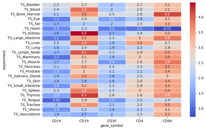
And there you have it! You have successfully performed a distributed operation on your single-cell data using TileDB Cloud’s serverless compute platform. This is just the tip of the iceberg in terms of what you can do with TileDB Cloud’s task graphs but should provide a good starting point for building more complex workflows.

Tip

See the Task Graphs section of Academy to learn more.

Housekeeping

Don’t forget to clean up after yourself! You can delete the UDF you registered to avoid cluttering your TileDB Cloud workspace.

tiledb.cloud.udf.delete(f"tiledb://{NAMESPACE}/soma_gene_stats")
Data Access
Basic S3 Example